Alireza Haghi Aghkand1*
1University of Qom, Qom, Iran
*Alireza_h378@yahoo.com
Abstract
Cubic equations are foundational in engineering and science, yet conventional solution methods—such as Cardano’s formula and Lagrange’s resolvent—are often computationally complex, numerically unstable or difficult to generalize. To address these limitations, this article introduced a novel Derivative Method (D-Method) for solving cubic equations by systematically reducing them to quadratic forms via derivative-based substitutions. The D-Method provided a closed-form solution for deriving at least one real root of any cubic equation, combining simplicity, accuracy and broad applicability to equations with real or complex coefficients. Unlike classical approaches, the method avoided intricate algebraic manipulations and memorization of cumbersome formulas, streamlining both manual and computational solving. Comparative analysis demonstrated that the D-Method outperformed traditional techniques in efficiency and accessibility. The solution’s validity was rigorously proved mathematically and illustrated through numerical examples. Furthermore, the method’s underlying framework suggested potential extensions to higher-degree polynomial equations, offering a pathway for future research.
Introduction
The history of cubic equations involves contributions from ancient Babylonian geometric methods, Greek explorations of conic sections, Islamic mathematicians' systematic approaches and significant advancements during the European Renaissance. The modern understanding was shaped by the algebraic insights of mathematicians like Descartes, Abel and Galois. These references provide a comprehensive view of the development of cubic equations over time.
Ancient and Medieval Contributions
Recent archaeological and mathematical studies confirm that the Babylonian mathematicians (c. 1800–1600 BCE) used iterative methods to approximate cubic roots. Robson (2008) analyzed cuneiform tablets (e.g., BM 85200) that solved problems equivalent to cubic equations for practical applications like volume calculations.
The Greeks, particularly Archimedes (3rd century BCE), encountered cubics in geometric problems, such as doubling the cube. However, as Netz (2022) noted, their solutions remained geometric rather than algebra, that is reflecting the limitations of their mathematical framework.
Omar Khayyam (1048–1131) classified cubic equations into 14 types (excluding negative coefficients) and solved them using intersecting conics. Recent work by Berggren (2016) reevaluates Khayyam’s methods, arguing that his approach was more systematic than previously thought, though still lacks a general formula.
The Renaissance Breakthrough: Algebraic Solutions in Italy
In the early 16th century, Scipione del Ferro (1465–1526) solved the depressed cubic $x^3+px=q$. According to recent research by Maracchia (2020), del Ferro likely kept his solution secret due to the competitive academic environment of Bologna.
Niccolò Tartaglia (1500–1557) said that we need to solve the cubic independently in 1535. A 2019 study by Gavagna revisited Tartaglia’s notebooks, suggesting he may have had access to del Ferro’s earlier work but potentially refined the method independently.
Gerolamo Cardano (1501–1576) published the general solution in Ars Magna (1545), crediting del Ferro and Tartaglia but violating an oath of secrecy. Recent historiography (Zetterberg, 2021) argues that Cardano’s publication was less an act of betrayal and more an effort to systematize mathematical knowledge.
Cardano’s student, Lodovico Ferrari (1522–1565), extended the method to quartic equations. Bussotti (2023) highlights how Ferrari’s work demonstrated the growing interconnectedness of polynomial solutions.
Post-Renaissance Developments
François Viète (1540–1603) introduced trigonometric identities to solve irreducible cubics (those with three real roots). A 2022 study by Goldstein demonstrated how Vieta’s approach bridged algebra and geometry.
Rafael Bombelli (1526–1572) explored complex numbers in cubic solutions. Recent analysis (Mazzotti, 2021) reexamined Bombelli’s L’Algebra (1572), arguing that his treatment of imaginary numbers was more rigorous than previously acknowledged.
Modern Perspectives
Contemporary historians (e.g., La Nave 2020) emphasizes that the cubic’s solution was not just a mathematical milestone but also a cultural shift marking the transition from geometric to symbolic algebra. Computational studies (Petrillo 2023) now model historical solution methods, revealing their efficiency and limitations.
Objectives and Structure
The primary limitation of existing methods lies in their lack of simplicity and generalizability, particularly for manual computation. This creates a need for a more straightforward and accurate approach to solve the cubic equations. To address this gap, we propose the Derivative Method (D-Method), which leverages derivatives and substitutions to transform a cubic equation into a quadratic form, enabling the derivation of a closed-form solution for one of its roots. This method aims to simplify the solving process, reduce computational complexity and provides a generalizable framework applicable to cubic equations with real or complex coefficients.
The objectives of this study are threefold: (1) to introduce the D-Method as a novel approach for solving cubic equations, (2) to demonstrate its application through illustrative examples and (3) to validate its accuracy and generality through mathematical proof. By focusing on simplicity and practicality, the D-Method offers a valuable alternative to traditional techniques, with potential extensions to higher-degree polynomials.
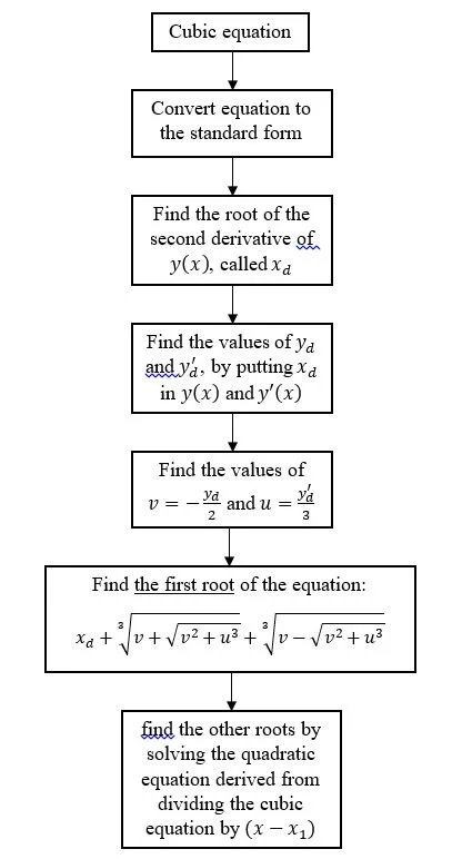
The structure of the paper is as follows: Section 2 explains the D-Method procedure. In Section 3, we present an example to demonstrate how the D-Method can be used to solve a cubic equation. We also compare it with four major methods, including Cardano's method, Vieta's substitution, Lagrange's resolvent and the trigonometric solution. Section 4 derives the D-Method's formula, while Section 5 verifies the solution through direct substitution. Section 6 shows that the D-Method can also be applied to quadratic equations. Section 7 discusses advantages and disadvantages of various methods. Finally, Section 8 concludes the paper. A schematic flowchart of the steps involved in solving the equation using the proposed method is provided in the appendix.
Explaining the D-Method Procedure
Consider the following equation as the standard general form of a cubic equation:
$$ x^3 + ax^2 + bx + c = 0 $$
In which $a$, $b$, and $c$ are arbitrary complex numbers. Since the left side of the equation is a cubic function, we can call it $y(x)$ (1):
$$ y(x) = x^3 + ax^2 + bx + c $$
Now we can find the roots of the above equation through the following five steps:
1. Finding the root of the second derivative of $y(x)$, which is called $x_d$:
$$ y’’(x) = 0 \rightarrow x = x_d $$
2. Finding the values of $y_d$ and $y’_d$ by putting $x_d$ in $y(x)$ and $y’(x)$:
$$ y_d = y(x_d), y’d = y’(x_d) $$
3. Finding the values of $v$ and $u$:
$$ v = -\frac{1}{2}y_d , u = \frac{1}{3} y’_d $$
4. Finding the first root of the equation from the following formula (2):
$$ x_1 = x_d + \sqrt[3]{v+sqrt(v^2+u^3)} + \sqrt[3]{v-sqrt(v^2+u^3)} $$
According to the fundamental theorem of algebra, a polynomial of degree 3 has exactly 3 roots. So how can we get the other two roots of the above cubic equation? The answer is to use the division of algebraic expressions:
5. We can rewrite any general cubic equation in form of $(x-x_1)(x-x_1)(x-x_3)=0$, where $x_1$, $x_2$, and $x_3$ are the roots of the equation. So if we know one of the roots of the cubic equation (for example $x_1$), we can find the other roots by solving the quadratic equation obtained from dividing the cubic equation by $(x-x_1)$:
$$ \frac{y(x)}{(x-x_1)} = 0 \rightarrow x = x_2 \ x = x_3 $$
So to summarize, first we find one of the roots of the cubic equation using the differential method (above formula) and then, we find the remaining roots by division of algebraic expressions.
Case Study and Comparison With Other Major Methods
To understand how this method works and appreciate its advantages, we study a detailed example in this section. We also compare it with several major methods.
Consider the following cubic equation:
$$ 2x^3 - 4x^2 - 2x + 4 = 0$$
The D-Method
First, we need to convert the equation into the standard form (in which the coefficient of $x^3$ is one):
$$2x^3-4x^2-2x+4=) \div 2 \rightarrow x^3-2x^2 - x + 2 = 0 $$
Then we can start solving the equation step by step as follows:
The first step is to find $x_d$:
$$ y(x) = x^3 - 2x^2 - x + 2 \Rightarrow y’(x) = 3x^2 - 4x - 1 y’’(x) = 6x - 4$$
$$ y’’(x) = 6x - 4 = 0 \Rightarrow x_d = \frac{4}{6}=\frac{2}{3} $$
The second step is to find $y_d$ and $y’_d$:
$$ y(x_d) = y_d = (\frac{2}{3})^3 - 2 (\frac{2}{3})^2 - (\frac{2}{3}) + 2 = \frac{20}{27}y’(x_d)=y’_d = 3(\frac{2}{3})^2 - 4(\frac{2}{3}) - 1 = -\frac{7}{3}$$
The third step is to find y_d and y’_d:
$$ v=-\frac{1}{2}y_d = -\frac{10}{27}u = \frac{1}{3}y’_d = -\frac{7}{9} $$
Now we can use the formula to find the first root:
$$ x_1 = x_d + \sqrt[3]{v+\sqrt(v^2 + u^3)} + \sqrt[3]{v-\sqrt(v^2+u^3)} $$
$$ \Rightarrow x_1 = \frac{2}{3} + \sqrt[3]{-\frac{10}{27}+\sqrt{(-\frac{10}{27})^2+(-\frac{7}{9})^3}} + \sqrt[3]{-\frac{10}{27}-\sqrt{(-\frac{10}{27})^2 + (-\frac{7}{9})^3}} $$
We can simplify the above root:
$$x_1 = \frac{2}{3}+\sqrt[3]{-\frac{10}{27}+\sqrt{\frac{100}{729}-\frac{343}{729}}} + \sqrt[3]{-\frac{10}{27}-\sqrt{\frac{100}{729}-\frac{343}{729}}} $$
$$ = \frac{2}{3} + \sqrt[3]{-\frac{10}{27}+\frac{\sqrt{-243}}{27}} + \sqrt[3]{-\frac{10}{27}-\frac{\sqrt{-243}}{27}} $$
Here we have two nested radicals which must be denested. Simply, we can say that
$Since (2+\sqrt{-3})^3 = -10+9\sqrt{-3}$ $(2-\sqrt{-3})^3 = -10-9\sqrt{-3}$
$Then \sqrt[3]{-10+9\sqrt{-3}} = 2+\sqrt{-3}$ $\sqrt[3]{-10-9\sqrt{-3}} = 2-\sqrt{-3}$
But there is also a simple approach to find the denested forms. If we write the nested radicals as
$$\sqrt[3]{-10+9\sqrt{-3}} = a + b\sqrt{-3}$ $\sqrt[3]{-10-9\sqrt{-3}} = a - b\sqrt{-3}$$
And multiply the left sides and the right sides to each other
$$\sqrt[3]{(-10+9\sqrt{-3})(-10-9\sqrt{-3})} = (a+b\sqrt{-3})(a-b\sqrt{-3})$$
$$\sqrt[3]{(-10)^2 - (9\sqrt{-3})^2} = a^2 - (b\sqrt{-3})^2$$
$$\sqrt[3]{100 - 81(-3)} = a^2 - b^2(-3) \rightarrow a^2 + 3b^2 = 7$$
We reach the above equation between $a$ and $b$. But we need another equation too, since we have two unknowns. We can use one of the above nested radicals
$$\sqrt[3]{-10+9\sqrt{-3}} = a + b\sqrt{-3} \rightarrow -10+9\sqrt{-3} = (a+b\sqrt{-3})^3$$
$$a^3 + 3a^2b\sqrt{-3} + 3a(b\sqrt{-3})^2 + (b\sqrt{-3})^3 = -10+9\sqrt{-3}$$
$$(a^3 - 9ab^2) + (3a^2b - 3b)\sqrt{-3} = -10+9\sqrt{-3}$$
$$\rightarrow a^3 - 9ab^2 = -10 \quad 3a^2b - 3b^3 = 9$$
Now we have three equations between $a$ and $b$. It's enough to guess the values of $a$ and $b$ which satisfies the above equation.
$$ 1. a = \pm 2, \; b = \pm 1 \rightarrow a^2 + 3b^2 = 4 + 3 = 7$$
$$ 2. a = +2, \; b = \pm 1 \rightarrow a^3 - 9ab^2 = 8 - 18 = -10 \quad \rightarrow a = +2$$
$$ 3. a = +2, \; b = +1 \rightarrow 3a^2b - 3b^3 = 12 - 3 = 9 \quad \rightarrow b = +1$$
Thus
$$\sqrt[3]{-10 + 9\sqrt{-3}} = a + b\sqrt{-3} = 2 + \sqrt{-3} \quad \sqrt[3]{-10 - 9\sqrt{-3}} = a - b\sqrt{-3} = 2 - \sqrt{-3}$$
By putting the denested radicals in the first root expression, we can simplify it as follows:
$$x_1 = \frac{2}{3} + \frac{\sqrt[3]{-10 + 9\sqrt{-3}}}{3} + \frac{\sqrt[3]{-10 - 9\sqrt{-3}}}{3} =$$
$$\frac{2}{3} + \frac{2 + \sqrt{-3}}{3} + \frac{2 - \sqrt{-3}}{3}$$
$$x_1 = \frac{2 + 2 + \sqrt{-3} + 2 - \sqrt{-3}}{3} = \frac{3 \times 2}{3} \rightarrow x_1 = 2$$
Other roots can found by dividing $y(x)$ by $(x - x_1)$:
$$\frac{y(x)}{(x - x_1)} = \frac{2x^3 - 4x^2 - 2x + 4}{x - 2} = 2x^2 - 2$$
$$2x^2 - 2 = 0 \Rightarrow x_2 = 1 \quad x_3 = -1$$
So the roots of our cubic equation are $2$, $1$ and $-1$. By putting these numbers in the main equation, we can ensure that our answers are correct.
To compare the D-Method with other general analytical approaches, we now apply these methods to our example. First, however, we must clarify what a depressed equation is.
Depressed cubic
Cubics of the form $t^3 + pt + q$ are said to be depressed. They are much simpler than general cubics, but are fundamental, because the study of any cubic may be reduced by a simple change of variable to that of a depressed cubic.
Let $ax^3 + bx^2 + cx + d = 0$ be a cubic equation. The change of variable $x = t - \frac{b}{3a}$ gives a cubic (in $t$) that has no term in $t^2$.
After dividing by $a$ we obtain the depressed cubic equation $t^3 + pt + q = 0$ with $t = x + \frac{b}{3a}$.
For the case $2x^3 - 4x^2 - 2x + 4 = 0$, the depressed form of the equation is
$$x = t - \frac{(-4)}{3(2)} = t + \frac{2}{3} \rightarrow 2\left(t + \frac{2}{3}\right)^3 - 4\left(t + \frac{2}{3}\right)^2$$
$$- 2\left(t + \frac{2}{3}\right) + 4 = 0 \rightarrow t^3 - \frac{7}{3}t + \frac{20}{27} = 0$$
Cardano's Method
This method applies to a depressed cubic $t^3 + pt + q = 0$. The idea is to introduce two variables $u$ and $v$ such that $u + v = t$ and to substitute this in the depressed cubic, giving
$$(u^3 + v^3) + (3uv + p)(u + v) + q = 0$$
Cardano's method proceeds by imposing the condition $3uv + p = 0$ which removes the third term in previous equality, leading to the system of equations
$$u^3 + v^3 = -q \quad uv = -\frac{p}{3}$$
Given the sum and the product of $u^3$ and $v^3$, one deduces that they are the two solutions of the quadratic equation
$$(z - u^3)(z - v^3) = z^2 - (u^3 + v^3)z + u^3v^3 = 0$$
So $z^2 + qz - \frac{p^3}{27} = 0$. The solutions to this equation are
$$-\frac{q}{2} \pm \sqrt{\frac{q^2}{4} + \frac{p^3}{27}}$$
resulting in
$$u = \sqrt[3]{-\frac{q}{2} + \sqrt{\frac{q^2}{4} + \frac{p^3}{27}}} \quad \& \quad v = \sqrt[3]{-\frac{q}{2} - \sqrt{\frac{q^2}{4} + \frac{p^3}{27}}}$$
As $t = u + v$. The sum of these solutions is a root of the original equation. That is
$$t = \sqrt[3]{-\frac{q}{2} + \sqrt{\frac{q^2}{4} + \frac{p^3}{27}}} + \sqrt[3]{-\frac{q}{2} - \sqrt{\frac{q^2}{4} + \frac{p^3}{27}}}$$
is a root of the equation. This is known as Cardano's formula.
The other roots of the equation can be obtained by multiplying the cube root by the two primitive cube roots of unity, which are $\omega = \frac{-1 + \sqrt{-3}}{2}$ and $\omega^2 = \frac{-1 - \sqrt{-3}}{2}$.
In case of our example, with depressed form of $t^3 - \frac{7}{3}t + \frac{20}{27} = 0$, the Cardano's solution is as follows:
Introducing two variables $u$ and $v$ such that $u + v = t$ and substituting this in the depressed cubic, gives
$$t = u + v \rightarrow t^3 = (u + v)^3 = u^3 + v^3 + 3uv(u + v)$$
$$\rightarrow t^3 - (3uv)t - (u^3 + v^3) = 0$$
Then we have
$$-(3uv) = -\frac{7}{3} \quad \& \quad -(u^3 + v^3) = \frac{20}{27}$$
$$\rightarrow uv = \frac{7}{9} \rightarrow u^3v^3 = \frac{343}{729} u^3 + v^3 = -\frac{20}{27}$$
Given the product $uv$ and sum of $u^3$ and $v^3$, we can find their values by considering them as the roots of a quadratic equation as follows:
$$t^2 - (u^3 + v^3)t + (uv) = 0$$
As a result, for the above example, we have
$$z^2 - (u^3 + v^3)z + u^3v^3 = 0 \rightarrow z^2 + \frac{20}{27}z + \frac{343}{729} = 0$$
$$z_1 = u^3 = \frac{-10 + 9\sqrt{-3}}{27} \quad \& \quad z_2 = v^3 = \frac{-10 - 9\sqrt{-3}}{27}$$
$$\rightarrow u = \frac{\sqrt[3]{-10 + 9\sqrt{-3}}}{3} \quad \& \quad v = \frac{\sqrt[3]{-10 - 9\sqrt{-3}}}{3}$$
Simplifying the two nested radicals appearing in the above roots gives:
$$\sqrt[3]{-10 + 9\sqrt{-3}} = 2 + \sqrt{-3} \quad \sqrt[3]{-10 - 9\sqrt{-3}} = 2 - \sqrt{-3}$$
Therefore
$$u = \frac{2 + \sqrt{-3}}{3} \quad \& \quad v = \frac{2 - \sqrt{-3}}{3}$$
and $t$ is obtained as
$$t = u + v = \frac{2 + i\sqrt{3}}{3} + \frac{2 - i\sqrt{3}}{3} = \frac{4}{3}$$
Finally, the value of the first root of the equation, $x_1$, is equal to
$$x_1 = t + \frac{2}{3} = \frac{4}{3} + \frac{2}{3} = \frac{6}{3} = 2$$
**To calculate other roots, one of the following two methods can be used:**
Method 1) The other two roots are obtained by dividing the original equation by $(x - x_1)$ and solving the resulting quadratic equation:
$$\frac{2x^3 - 4x^2 - 2x + 4}{x - 2} = 2x^2 - 2 = 0 \rightarrow (x^2 - 1) = 0 \rightarrow x_2 = 1 \quad x_3 = -1$$
Method 2) If one of the roots of the depressed equation is $t = u + v$, then its other two roots are:
$$t = \omega u + \omega^2 v \quad t = \omega^2 u + \omega v$$
where $\omega$ and $\omega^2$ are the primitive cube roots of unity, i.e.
$$\omega = \frac{-1 + \sqrt{-3}}{2} \rightarrow \omega^2 = \frac{-1 - \sqrt{-3}}{2}$$
Therefore
$$\omega u + \omega^2 v = \frac{-(u + v) + (u - v)\sqrt{-3}}{2} \quad \& \quad \omega^2 u + \omega v = \frac{-(u + v) - (u - v)\sqrt{-3}}{2}$$
For the depressed equation of the example above, we have:
$$u + v = \frac{2 + \sqrt{-3}}{3} + \frac{2 - i\sqrt{3}}{3} = \frac{4}{3} \quad \& \quad u - v = \frac{2 + \sqrt{-3}}{3} - \frac{2 - i\sqrt{3}}{3} = \frac{2i\sqrt{3}}{3}$$
$$\rightarrow \omega u + \omega^2 v = \frac{-\left(\frac{4}{3}\right) + i\left(\frac{2i\sqrt{3}}{3}\right)\sqrt{3}}{2} = -\frac{5}{3} \quad \&$$
$$\omega^2 u + \omega v = \frac{-\left(\frac{4}{3}\right) - i\left(\frac{2i\sqrt{3}}{3}\right)\sqrt{3}}{2} = \frac{1}{3}$$
Thus, the roots of the general equation are:
$$x = t + \frac{2}{3}$$
$$\rightarrow t_1 = u + v \rightarrow x_1 = \frac{2}{3} + \frac{4}{3} = 2$$
$$t_2 = \omega u + \omega^2 v \rightarrow x_2 = \frac{2}{3} - \frac{5}{3} = -1$$
$$t_3 = \omega^2 u + \omega v \rightarrow x_3 = \frac{2}{3} + \frac{1}{3} = 1$$
As observed, Cardano's method is comprehensive but lengthy and requires many steps to arrive at the answer.
Vieta's Substitution
Starting from the depressed cubic $t^3 + pt + q = 0$, Vieta's method substitutes $t$ with $w - \frac{p}{3w}$. The substitution transforms the depressed cubic into
$$w^3 + q - \frac{p^3}{27w^3} = 0$$
Multiplying by $w^3$, we obtain a quadratic equation in $w^3$:
$$(w^3)^2 + q(w^3) - \frac{p^3}{27} = 0$$
Let
$$W = -\frac{q}{2} \pm \sqrt{\frac{q^2}{4} + \frac{p^3}{27}}$$
be any nonzero root of this quadratic equation. If $w_1$, $w_2$ and $w_3$ are the three cube roots of $W$, then the roots of the original depressed cubic are $w_1 - \frac{p}{3w_1}$, $w_2 - \frac{p}{3w_2}$ and $w_3 - \frac{p}{3w_3}$. The other root of the quadratic equation is $-\frac{p^3}{27W}$. This implies that changing the sign of the square root exchanges $w_i$ and $-\frac{p^3}{27w_i}$ for $i = 1, 2, 3$ and therefore does not change the roots.
In case of our example, with depressed form of $t^3 - \frac{7}{3}t + \frac{20}{27} = 0$, the Vieta's substitution is as follows:
Vieta's substitution, $t = w - \frac{p}{3w}$, transforms the depressed cubic into
$$t = w - \frac{p}{3w}$$
$$= w - \frac{\left(-\frac{7}{3}\right)}{3w}$$
$$= w + \frac{7}{9w}$$
$$\Rightarrow 2\left(w + \frac{7}{9w}\right)^3 - 4\left(w + \frac{7}{9w}\right)^2 - 2\left(w + \frac{7}{9w}\right) + 4 = 0$$
$$\rightarrow w^3 + \frac{20}{27} - \frac{343}{729 w^3} = 0$$
Multiplying by $w^3$, we obtain a quadratic equation in $w^3$:
$$(w^3)^2 + \frac{20}{27} (w^3) - \frac{343}{729} = 0$$
The roots of the above quadratic equation are:
$$w^3 = \frac{-10 \pm 9\sqrt{-3}}{27} \rightarrow w = \frac{\sqrt[3]{-10 \pm 9\sqrt{-3}}}{3}$$
Simplifying the two nested radicals appearing in the roots above:
$$w = \frac{\sqrt[3]{-10 \pm 9\sqrt{-3}}}{3} = \frac{2 \pm \sqrt{-3}}{3}$$
As a result, $t$ is obtained as
$$t = w - \frac{p}{3w} = \frac{2 \pm \sqrt{-3}}{3} - \frac{\left(-\frac{7}{3}\right)}{3\left(\frac{2 \pm \sqrt{-3}}{3}\right)} = \frac{4}{3}$$
and the value of the first root of the equation, $x_1$, is equal to
$$x_1 = t + \frac{2}{3} = \frac{4}{3} + \frac{2}{3} = \frac{6}{3} = 2$$
The other two roots are obtained by dividing the original equation by $(x - x_1)$ and solving the resulting quadratic equation:
$$\frac{2x^3 - 4x^2 - 2x + 4}{x - 2} = 2x^2 - 2 = 0 \rightarrow (x^2 - 1) = 0 \rightarrow x_2 = 1 \quad x_3 = -1$$
Lagrange's Method
Lagrange's main idea was to work with the discrete Fourier transform of the roots instead of the roots themselves. More precisely, let $\omega$ be a primitive third root of unity, that is a
number such that $\omega^3 = 1$ and $\omega^2 + \omega + 1 = 0$. Denoting $x_0$, $x_1$ and $x_2$ the three roots of the cubic equation to be solved and let
$$s_0 = x_0 + x_1 + x_2 \quad s_1 = x_0 + \omega x_1 + \omega^2 x_2 \quad s_2 = x_0 + \omega^2 x_1 + \omega x_2$$
be the discrete Fourier transform of the roots. If $s_0$, $s_1$ and $s_2$ are known, the roots using the inverse Fourier transform, which involves inverting the corresponding linear transformation. That is
$$x_0 = \frac{1}{3}(s_0 + s_1 + s_2) \quad x_1 = \frac{1}{3}(s_0 + \omega s_1 + \omega^2 s_2) \quad x_2 = \frac{1}{3}(s_0 + \omega^2 s_1 + \omega s_2)$$
By Vieta's formulas, $s_0$ is known to be zero in the case of a depressed cubic and $-\frac{b}{a}$ for the general cubic. So, only $s_1$ and $s_2$ need to be computed. They are not symmetric functions of the roots (swapping $x_1$ and $x_2$ also swaps $s_1$ and $s_2$), but some simple symmetric functions of $s_1$ and $s_2$ are also symmetric in the roots of the cubic equation to be solved. Thus these symmetric functions can be expressed in terms of the (known) coefficients of the original cubic and this allows eventually expressing the $s_i$ as roots of a polynomial with known coefficients.
In the case of a cubic equation, $P = s_1 s_2$ and $S = s_1^3 + s_2^3$ are such symmetric polynomials (see below). It follows that $s_1^3$ and $s_2^3$ are the two roots of the quadratic equation $z^2 - Sz + P^3 = 0$.
Computation of $S$ and $P$
A straightforward computation using the relations $\omega^3 = 1$ and $\omega^2 + \omega + 1 = 0$ gives
$$P = s_1 s_2 = x_0^2 + x_1^2 + x_2^2 - (x_0 x_1 + x_1 x_2 + x_2 x_0)$$
$$S = s_1^3 + s_2^3 = 2\left(x_0^3 + x_1^3 + x_2^3\right) - 3\left(x_0^2 x_1 + x_1^2 x_2 + x_2^2 x_0 + x_0 x_1^2 + x_1 x_2^2 + x_2 x_0^2\right) + 12x_0 x_1 x_2$$
This shows that $P$ and $S$ are symmetric functions of the roots. Using Newton's identities, it is straightforward to express them in terms of the elementary symmetric functions of the roots, giving
$$P = e_1^2 - 3e_2 \quad S = 2e_1^3 - 9e_1 e_2 + 27e_3$$
with $e_1 = 0$, $e_2 = p$ and $e_3 = -q$ in the case of a depressed cubic and $e_1 = -\frac{b}{a}$, $e_2 = \frac{c}{a}$ and $e_3 = -\frac{d}{a}$, in the general case.
In case of our example, with depressed form of $t^3 - \frac{7}{3}t + \frac{20}{27} = 0$, the Lagrange's solution is as follows
Denoting $t_0$, $t_1$ and $t_2$ the three roots of the depressed cubic equation to be solved, let
$$s_0 = t_0 + t_1 + t_2 \quad s_1 = t_0 + \omega t_1 + \omega^2 t_2 \quad s_2 = t_0 + \omega^2 t_1 + \omega t_2$$
be the discrete Fourier transform of the roots. If $s_0$, $s_1$ and $s_2$ are known, the roots may be recovered from them with the inverse Fourier transform consisting of inverting this linear transformation
$$t_0 = \frac{1}{3}(s_0 + s_1 + s_2)$$
$$t_1 = \frac{1}{3}(s_0 + \omega s_1 + \omega^2 s_2)$$
$$t_2 = \frac{1}{3}(s_0 + \omega^2 s_1 + \omega s_2)$$
$s_0$ is known to be zero in the case of a depressed cubic. So, only $s_1$ and $s_2$ need to be computed. In the case of a cubic equation, $P = s_1 s_2$ and $S = s_1^3 + s_2^3$ are symmetric polynomials. It follows that $s_1^3$ and $s_2^3$ are the two roots of the quadratic equation $z^2 - Sz + P^3 = 0$ and in the case of a depressed cubic, $t^3 + pt + q = 0$, they can be calculated as
$$P = -3p = -3 \times -\frac{7}{3} = 7 \quad S = -27q = -27 \times \frac{20}{27} = -20$$
As a result, the quadratic equation becomes:
$$z^2 + 20z + 343 = 0$$
whose roots are:
$$z_1 = s_1^3 = -10 + 9\sqrt{-3}$$
$$z_2 = s_2^3 = -10 - 9\sqrt{-3}$$
$$\Rightarrow s_1 = \sqrt[3]{-10 + 9\sqrt{-3}} = 2 + \sqrt{-3}$$
$$s_2 = \sqrt[3]{-10 - 9\sqrt{-3}} = 2 - \sqrt{-3}$$
Thus, the roots of the depressed equation are
$$t_0 = \frac{1}{3}(s_0 + s_1 + s_2)$$
$$= \frac{(2 + \sqrt{-3}) + (2 - \sqrt{-3})}{3}$$
$$= \frac{4}{3}$$
$$t_1 = \frac{1}{3}(s_0 + \omega s_1 + \omega^2 s_2)$$
$$= \frac{\omega(2 + \sqrt{-3}) + \omega^2(2 - \sqrt{-3})}{3}$$
$$= -\frac{5}{3}$$
$$t_2 = \frac{1}{3}(s_0 + \omega^2 s_1 + \omega s_2)$$
$$= \frac{\omega^2(2 + \sqrt{-3}) + \omega(2 - \sqrt{-3})}{3}$$
$$= \frac{1}{3}$$
and finally, the roots of the general equation are:
$$x = t + \frac{2}{3} \rightarrow t_0 = u + v \rightarrow x_0 = \frac{2}{3} + \frac{4}{3} = 2$$
$$t_1 = \omega u + \omega^2 v \rightarrow x_1 = \frac{2}{3} - \frac{5}{3} = -1$$
$$t_2 = \omega^2 u + \omega v \rightarrow x_2 = \frac{2}{3} + \frac{1}{3} = 1$$
Trigonometric Solution
Galois theory shows that when the three roots are real and none is rational (*Casus irreducibilis*), the roots cannot be expressed in terms of real radicals. Nevertheless, purely real expressions of the solutions can be obtained using trigonometric functions, specifically in terms of cosines and arccosines. More precisely, the roots of the depressed cubic $t^3 + pt + q = 0$ are
$$t_k = 2\sqrt{-\frac{p}{3}} \cos \left( \frac{1}{3} \arccos \left( \frac{3q}{2p} \sqrt{-\frac{3}{p}} \right) - \frac{2k\pi}{3} \right), \quad k = 0, 1, 2$$
This formula, attributed to François Viète, yields a purely real expression when the cubic equation has three real roots that is, when $4p^3 + 27q^2 < 0$. In cases where there is only one real root, the formula remains mathematically valid but involves complex-valued cosine and arccosine functions. However, when $p = 0$ the formula becomes undefined due to a division by zero.
The formula can be proved as follows: Starting from the equation $t^3 + pt + q = 0$, let us set $t = u \cos \theta$. The idea is to choose $u$ to make the equation coincide with the identity
$$4\theta - 3\cos \cos\theta - \cos\cos(3\theta) = 0$$
Choosing $u = 2\sqrt{-\frac{p}{3}}$ and dividing the equation by $\frac{u^3}{4}$ gives
$$4\theta - 3\cos \cos\theta - \frac{3q}{2p}\sqrt{-\frac{3}{p}} = 0$$
Then combining with the above identity, we obtain
$$\cos\cos(3\theta) = \frac{3q}{2p}\sqrt{-\frac{3}{p}}$$
resulting in
$$t_k = 2\sqrt{-\frac{p}{3}} \cos \left( \frac{1}{3} \arccos \left( \frac{3q}{2p} \sqrt{-\frac{3}{p}} \right) - \frac{2k\pi}{3} \right), \quad k = 0, 1, 2$$
In case of our example, with depressed form of $t^3 - \frac{7}{3}t + \frac{20}{27} = 0$, the trigonometric solution is as follows
let us set $t = u \cos \theta$
$$(u \cos \theta)^3 - \frac{7}{3}(u \cos \theta) + \frac{20}{27} = 0 \Rightarrow$$
$$\cos^3 \theta - \frac{7}{3u^2} \cos \theta + \frac{20}{27u^3} = 0$$
Comparing the above equation with the following trigonometric identity
$$\cos(3\theta) = 4 \cos^3 \theta - 3 \cos \theta \Rightarrow$$
$$\cos^3 \theta - \frac{3}{4} \cos \theta - \frac{1}{4} \cos(3\theta) = 0$$
gives
$$-\frac{7}{3u^2} = -\frac{3}{4} \Rightarrow u^2 = \frac{28}{9} \Rightarrow u = \frac{2}{3}\sqrt{7}$$
$$\frac{20}{27u^3} = -\frac{1}{4} \cos(3\theta)$$
$$\Rightarrow \cos(3\theta) = -\frac{80}{27u^3} = -\frac{10}{49}\sqrt{7}$$
$$\Rightarrow \theta = \frac{1}{3} \arccos \left( -\frac{10}{49}\sqrt{7} \right)$$
So, we can find the root of the depressed equation as
$$t = u \cos \theta = \frac{2}{3}\sqrt{7} \times \frac{1}{3} \arccos \left( -\frac{10}{49}\sqrt{7} \right)$$
This is consistent with the equation mentioned above for calculating the roots:
$$t_k = 2\sqrt{-\frac{p}{3}} \cos \left( \frac{1}{3} \arccos \left( \frac{3q}{2p} \sqrt{-\frac{3}{p}} \right) - \frac{2k\pi}{3} \right), \quad k = 0, 1, 2$$
Thus
$$k = 0 \Rightarrow t_0 = 2\sqrt{-\frac{p}{3}} \cos \left( \frac{1}{3} \arccos \left( \frac{3q}{2p} \sqrt{-\frac{3}{p}} \right) \right) = 1.3333$$
$$k = 1 \quad \Rightarrow \quad t_1 = 2\sqrt{-\frac{p}{3}} \cos \left( \frac{1}{3} \arccos \left( \frac{3q}{2p} \sqrt{-\frac{3}{p}} \right) - \frac{2\pi}{3} \right) = 0.3333$$
$$k = 2 \quad \Rightarrow \quad t_2 = 2\sqrt{-\frac{p}{3}} \cos \left( \frac{1}{3} \arccos \left( \frac{3q}{2p} \sqrt{-\frac{3}{p}} \right) - \frac{4\pi}{3} \right) = -1.6667$$
Therefore, the roots of the original cubic equation are
$$x = t + \frac{2}{3} \quad \Rightarrow \quad t_0 = 1.3333 \quad \Rightarrow \quad x_0 = \frac{2}{3} + 1.3333 \approx 2$$
$$t_1 = 0.3333 \quad \Rightarrow \quad x_1 = \frac{2}{3} + 0.3333 \approx 1$$
$$t_2 = -1.6667 \quad \Rightarrow \quad x_2 = \frac{2}{3} - 1.6667 \approx -1$$
The Derivation of the D-Method Formula
Consider the general form of a cubic equation:
$$x^3 + ax^2 + bx + c = 0 \tag{1}$$
Since the left side of the equation is a cubic function, we can set it equal to a dependent variable say "$y$":
$$y(x) = x^3 + ax^2 + bx + c$$
Since this function is continuous, we can find the first and second derivatives of $y$:
$$\frac{dy}{dx} = y'(x) = 3x^2 + 2ax + b$$
$$\frac{d^2y}{dx^2} = y''(x) = 6x + 2a$$
The next step is to find the root of $y''$, which is a linear equation:
$$6x + 2a = 0 \Rightarrow 6x = -2a \Rightarrow x = \frac{-2a}{6} = -\frac{a}{3}$$
To distinguish it, we call this root "$x_d$":
$$x_d = -\frac{a}{3}$$
by putting $x_d$ in $y$ and its derivatives, we obtain:
$$y(x_d) = y_d = \left(-\frac{a}{3}\right)^3 + a\left(-\frac{a}{3}\right)^2 + b\left(-\frac{a}{3}\right) + c$$
$$= -\frac{a^3}{27} + \frac{3a^3}{27} - \frac{ab}{3} + c$$
$$= \frac{2a^3}{27} - \frac{ab}{3} + c$$
$$y'(x_d) = y'_d = 3\left(-\frac{a}{3}\right)^2 + 2a\left(-\frac{a}{3}\right) + b$$
$$= \frac{a^2}{3} - \frac{2a^2}{3} + b$$
$$= -\frac{a^2}{3} + b$$
$$y''(x_d) = y''_d = 6\left(-\frac{a}{3}\right) + 2a = -2a + 2a = 0$$
From this point onward, we use substitutions. First, we substitute $x = t + x_d$, to obtain the *depressed equation*:
$$x = t + x_d = t - \frac{a}{3} \quad \text{(general form)} \Rightarrow$$
$$\left(t - \frac{a}{3}\right)^3 + a\left(t - \frac{a}{3}\right)^2 + b\left(t - \frac{a}{3}\right) + c = 0$$
$$t^3 - 3t^2\left(\frac{a}{3}\right) + 3t\left(\frac{a}{3}\right)^2 - \left(\frac{a}{3}\right)^3 + a\left[t^2 - 2t\left(\frac{a}{3}\right) + \left(\frac{a}{3}\right)^2\right]$$
$$+ b\left(t - \frac{a}{3}\right) + c = 0$$
$$t^3 - at^2 + \frac{a^2}{3}t - \frac{a^3}{27} + at^2 - \frac{2a^2}{3}t + \frac{a^3}{9} + bt - \frac{ab}{3} + c = 0$$
$$t^3 + \left(-\frac{a^2}{3} + b\right)t + \left(\frac{2a^3}{27} - \frac{ab}{3} + c\right) = 0$$
$$t^3 + y'_dt + y_d = 0 \quad \text{(depressed equation)}$$
To convert the depressed equation into a quadratic equation, we substitute $t$ with $z - \frac{y'_d}{3z}$:
$$t = z - \frac{y'_d}{3z} \Rightarrow \left(z - \frac{y'_d}{3z}\right)^3 + y'_d\left(z - \frac{y'_d}{3z}\right) + y_d = 0$$
$$z^3 - 3z^2\left(\frac{y'_d}{3z}\right) + 3z \cdot \frac{(y'_d)^2}{9z^2} - \frac{(y'_d)^3}{27z^3} + y'_dz - \frac{(y'_d)^2}{3z} + y_d = 0$$
$$z^3 + \frac{(y'_d)^2}{3z} - \frac{(y'_d)^3}{27z^3} - \frac{(y'_d)^2}{3z} + y_d = 0$$
$$\times z^3 \quad \Rightarrow \quad z^6 + y_dz^3 - \left(\frac{y'_d}{3}\right)^3 = 0$$
Upon closer inspection, we can understand that this equation is a quadratic equation with respect to $z^3$:
$$(z^3)^2 + y_d(z^3) - \left(\frac{y'_d}{3}\right)^3 = 0 \quad \text{(quadratic equation)}$$
Now we can find one root of the above equation from the quadratic formula:
$$z^3 = \frac{-y_d + \sqrt{y_d^2 - 4 \times 1 \times -\left(\frac{y'_d}{3}\right)^3}}{2 \times 1}$$
$$= -\frac{y_d}{2} + \frac{\sqrt{y_d^2 + 4\left(\frac{y'_d}{3}\right)^3}}{2}$$
$$= -\frac{y_d}{2} + \sqrt{\frac{4\left(\frac{y_d^2}{4} + \left(\frac{y'_d}{3}\right)^3\right)}{4}}$$
$$\Rightarrow \quad z^3 = -\frac{y_d}{2} + \sqrt{\left(-\frac{y_d}{2}\right)^2 + \left(\frac{y'_d}{3}\right)^3}$$
To further simplify our work, we also introduce the following two substitutions:
$$v = -\frac{y_d}{2}, \quad u = \frac{y'_d}{3}$$
Hence
\[z^3=v+\sqrt{v^2+u^3} \quad \Rightarrow \quad z=\sqrt[3]{v+\sqrt{v^2+u^3}}\]
From the second substitution we conclude that:
\[t=z-\frac{y'_d}{3z}=z-\frac{(\frac{y'_d}{3})}{z}=z-\frac{u}{z}\]
\[\Rightarrow \quad t=\sqrt[3]{v+\sqrt{v^2+u^3}}-\frac{u}{\sqrt[3]{v+\sqrt{v^2+u^3}}}\]
We can simplify the above formula by simplifying the second term of the right side:
\[\frac{u}{\sqrt[3]{v+\sqrt{v^2+u^3}}}=\frac{u}{\sqrt[3]{v+\sqrt{v^2+u^3}}}\times1\]\[=\frac{u}{\sqrt[3]{v+\sqrt{v^2+u^3}}}\times\frac{\sqrt[3]{v-\sqrt{v^2+u^3}}}{\sqrt[3]{v-\sqrt{v^2+u^3}}}\]
\[=\frac{u\times\sqrt[3]{v-\sqrt{v^2+u^3}}}{\sqrt[3]{(v+\sqrt{v^2+u^3})}(v-\sqrt{v^2+u^3})}\]
\[=\frac{\sqrt[3]{u^3}\times\sqrt[3]{v-\sqrt{v^2+u^3}}}{\sqrt[3]{v^2-(\sqrt{v^2+u^3})^2}}\]
\[=\frac{\sqrt[3]{u^3(v-\sqrt{v^2+u^3})}}{\sqrt[3]{v^2-({v^2+u^3})}}\]
\[=\sqrt[3]{\frac{u^3(v-\sqrt{v^2+u^3})}{v^2-v^2-u^3}}\]
\[=\sqrt[3]{\frac{u^3(v-\sqrt{v^2+u^3})}{-u^3}}\]
\[=\sqrt[3]{-(v-\sqrt{v^2+u^3})}\]
\[=-\sqrt[3]{v-\sqrt{v^2+u^3}}\]
Therefore, we can rewrite $t$ in the form of:
\[t=\sqrt[3]{v+\sqrt{v^2+u^3}}-\frac{u}{\sqrt[3]{v+\sqrt{v^2+u^3}}}\]
\[=\sqrt[3]{v+\sqrt{v^2+u^3}}-(-\sqrt[3]{v-\sqrt{v^2+u^3}})\]
\[\Rightarrow \quad t=\sqrt[3]{v+\sqrt{v^2+u^3}}+\sqrt[3]{v-\sqrt{v^2+u^3}}\]
and from the first substitution, we can derive the root $x$:
\[x=x_d+t \quad \Rightarrow \quad x=x_d+\sqrt[3]{v+\sqrt{v^2+u^3}}+\sqrt[3]{v-\sqrt{v^2+u^3}}\]
That is exactly what we were looking for. It appears that we can find one of the roots of any cubic equation with this formula but to be certain, we can verify the formula by putting it in the equation. In the next section, we will do precisely that.
Checking the Validity of the Formula
To see if a number is truly the root of an equation or not, we can put it in the equation in place of $x$. In this section, we put the derived root in the equation to confirm its validity and correctness. The general form of equation is:
\[x^3+ax^2+bx+c=0\]
and the formula of root is:
\[x=x_d+\sqrt[3]{v+\sqrt{v^2+u^3}}+\sqrt[3]{v-\sqrt{v^2+u^3}}\]
According to (2), we can rewrite the formula in the following form to simplify our calculations:
\[x=x_d+\sqrt[3]{v+\sqrt{v^2+u^3}}-\frac{u}{\sqrt[3]{v+\sqrt{v^2+u^3}}}\]
To simplify our calculations further, we can substitute $\sqrt[3]{v+\sqrt{v^2+u^3}}$ with $m$:
\[x=x_d+m-\frac{u}{m}\]
Putting the root formula in the equation yields:
\[(x_d+m-\frac{u}{m})^3+a(x_d+m-\frac{u}{m})^2+b(x_d+m-\frac{u}{m})+c=0\]
We can expand each term separately and add them up to obtain
\[\text{i)} \quad (x_d+m-\frac{u}{m})^3=(x_d+(m-\frac{u}{m}))^3=x_d^3+3x_d^2(m-\frac{u}{m})+3x_d(m-\frac{u}{m})^2+(m-\frac{u}{m})^3\]
\[\text{ii)} \quad (x_d+m-\frac{u}{m})^2=(x_d+(m-\frac{u}{m}))^2=x_d^2+2x_d(m-\frac{u}{m})+(m-\frac{u}{m})^2\]
By putting above expressions in equation:
\[x_d^3+3x_d^2(m-\frac{u}{m})+3x_d(m-\frac{u}{m})^2+(m-\frac{u}{m})^3+ax_d^2+2ax_d(m-\frac{u}{m})+a(m-\frac{u}{m})^2+bx_d+b(m-\frac{u}{m})+c\]
\[\quad =(x_d^3+ax_d^2+bx_d+c)\]
\[\quad +(3x_d^2+2ax_d+b)(m-\frac{u}{m})\]
\[\quad+(3x_d+a)(m-\frac{u}{m})^2+(m-\frac{u}{m})^3\]
\[=y_d+y'_d(m-\frac{u}{m})+\frac{y''_d}{2}(m-\frac{u}{m})^2+(m-\frac{u}{m})^3\]
Since $y''_d=0$ and consequently $\frac{y''_d}{2}=0$, the above expression simplifies to
\[y_d+y'_d(m-\frac{u}{m})+(m-\frac{u}{m})^3\]
By replacing $y_d$ and $y'_d$ with their equal values:
\[v=-\frac{y_d}{2} \quad \Rightarrow\quad y_d=-2v, \quad u=\frac{y'_d}{3} \quad \Rightarrow\quad y'_d=3u\]
\[\quad \Rightarrow \quad y_d+y'_d(m-\frac{u}{m})+(m-\frac{u}{m})^3=\]
\[\quad \quad \quad -2v+3u(m-\frac{u}{m})+(m-\frac{u}{m})^3\]
\[=-2v+3um-3u(\frac{u}{m})+m^3-3m^2(\frac{u}{m})+3m(\frac{u^2}{m^2})-(\frac{u}{m})^3\]
\[=-2v+3um-3\frac{u^2}{m}+m^3-3um+3\frac{u^2}{m}-\frac{u^3}{m^3}\] \[=-2v+m^3-\frac{u^3}{m^3}\]
Replacing $m^3$ with its equivalent expression confirms our claim, as shown in the following steps:
\[m=\sqrt[3]{v+\sqrt{v^2+u^3}} \quad \Rightarrow \quad m^3\]\[=v+\sqrt{v^2+u^3}\]
\[\Rightarrow \quad -2v+m^3-\frac{u^3}{m^3}=-2v+(v+\sqrt{v^2+u^3})-\frac{u^3}{(v+\sqrt{v^2+u^3})}\]\[=-v+\sqrt{v^2+u^3}-\frac{u^3}{(v+\sqrt{v^2+u^3})}\]
\[\quad \quad =-v+\sqrt{v^2+u^3}-\frac{u^3}{(v+\sqrt{v^2+u^3})}\times1\]
\[=-v+\sqrt{v^2+u^3}-(\frac{u^3}{v+\sqrt{v^2+u^3}}\times\frac{v-\sqrt{v^2+u^3}}{v-\sqrt{v^2+u^3}})\]
\[\quad=-v+\sqrt{v^2+u^3}-\frac{u^3(v-\sqrt{v^2+u^3})}{v^2-(\sqrt{v^2+u^3})^2}\]
\[\quad=-v+\sqrt{v^2+u^3}-\frac{u^3(v-\sqrt{v^2+u^3})}{v^2-v^2-u^3}\]
\[\quad=-v+\sqrt{v^2+u^3}-\frac{u^3(v-\sqrt{v^2+u^3})}{-u^3}\]
\[\quad=-v+\sqrt{v^2+u^3}+v-\sqrt{v^2+u^3}=0\]
We can now conclude that our formula is applicable to any cubic equation with complex or real coefficients. In other words, it allows us to find one root of any cubic equation. Since every cubic equation has three roots, once we find the first root using the formula (e.g., $x=x_1$), we can divide the left-hand side of equation (1) by $(x-x_1)$ to obtain a quadratic equation. The roots of this quadratic are the remaining two roots of the original cubic equation.
D-Method for Solving Quadratic Equations
Consider the following equation as the general form of a quadratic equation:
\[x^2+ax+b=0\]
We know that the roots of this equation are:
\[x_1=\frac{-a+\sqrt{a^2-4b}}{2}\]\[=-\frac{a}{2}+\frac{\sqrt{a^2-4b}}{2}=-\frac{a}{2}+\sqrt{\frac{a^2-4b}{4}}\]
\[x_2=\frac{-a-\sqrt{a^2-4b}}2{}\]
\[\quad = -\frac{a}{2}-\frac{\sqrt{a^2-4b}}{2}=-\frac{a}{2}-\sqrt{\frac{a^2-4b}{4}}\]
The root of the first derivative of the left side of the quadratic equation is given by:
\[y(x)=x^2+ax+b \text{→} y'(x)=2x+a\]
\[y'(x)=0\text{→} 2x+a=0\text{→}x_d=-\frac{a}{2}\]
Putting $x_d$ in the main equation yields
\[y(x_d)=(-\frac{a}{2})^2+a(-\frac{a}{2})+b=\frac{a^2}{4}-\frac{a^2}{2}+b=\frac{4b-a^2}{4}=-(\frac{a^2-4b}{4})\]
A comparison between $y(x_d)$ and the roots shows that:
\[x_1=x_d+\sqrt{v} \quad x_2=x_d-\sqrt{v}\]
Here, $x_d$ is the roots of the first derivative of the equation, and $v=-y_d$.
Discussion of the Results
As shown, Cardano's method and Vieta's substitution require multiple algebraic substitutions, making them cumbersome and error-prone. Cardano's method can introduce complexity through the emergence of complex numbers in cases of Casus irreducibilis and Vieta’s substitution often involves solving cube roots, sometimes with complex numbers.
Lagrange’s method uses Fourier-transform-inspired techniques, which are abstract and difficult to memorize, making them less practical for quick, manual calculations.
In contrast, the D-Method offers simplicity by relying on straightforward derivative-based substitutions that are easy to memorize and apply. It avoids the multiple algebraic substitutions needed in Cardano’s and Vieta’s methods. Although it involves nested radicals, this complexity is manageable compared to the other methods.
The trigonometric method is beneficial for cubic equations with three real roots, avoiding nested radicals entirely. However, it only applies to equations with real coefficients (Casus irreducibilis) and requires knowledge of trigonometric identities and depressed cubic transformations. It also yields approximate solutions due to the cosine values involved.
In summary, the D-Method provides an accessible, derivative-based alternative that simplifies solving cubic equations, balancing ease of memorization and practical usability. The choice of method should ultimately depend on the specific characteristics and constraints of the problem.
Conclusion
The D-Method simplifies cubic equation solving by replacing memorized formulas with derivative-based substitutions, offering a universal, stable and manual-friendly approach. Unlike Vièta’s substitution (limited to depressed cubics) or the trigonometric method (restricted to real coefficients), the D-Method handles all cubic forms -real or complex- without numerical instability (Casus irreducibilis) or transcendental functions. While classical methods excel in theoretical generality (e.g., Lagrange for higher-degree polynomials), the D-Method prioritizes practical accessibility and algebraic simplicity, extending naturally to quadratics and potentially higher-order equations.
References
Berggren, J. L. (2016). ‘Episodes in the Mathematics of Medieval Islam’, Springer.
Bussotti, P. (2023). ‘The Italian Algebra of the Renaissance’, Birkhäuser.
Gavagna, V. (2019). ‘Tartaglia and the Cubic Equation: A Reassessment’, Historia Mathematica, 46, 1-15.
Goldstein, C. (2022). ‘Vieta’s Trigonometric Approach to Cubics’, Archive for History of Exact Sciences, 76(3), 301-324.
La Nave, F. (2020). ‘Cardano and the Solution of the Cubic: A Reinterpretation’, Annals of Science, 77(2), 145-167.
Maracchia, S. (2020). ‘The Algebra of Scipione del Ferro. Firenze University Press’.
Mazzotti, M. (2021). ‘Bombelli and the Birth of Complex Numbers’, Isis, 112(1), 23-42.
Netz, R. (2022). ‘A New History of Greek Mathematics’, Cambridge UP.
Petrillo, G. (2023). ‘Computational Analysis of Renaissance Cubic Solutions Journal of Humanistic Mathematics, 13(1), 45-68.
Robson, E. (2008). ‘Mathematics in Ancient Iraq: A Social History’,. Princeton UP.
Zetterberg, J. (2021). ‘Cardano’s Ars Magna: Between Secrecy and Publication’, Renaissance Quarterly, 74(4), 1123-1150.
Appendix
Schematic flowchart of the Derivative method: