Statistical Analysis of Rodent Body Weight Data is Robust to Departures from Normality in Historical National Toxicology Program Studies Dated 1980-2013

Alyssa M Taylor-Lapole, Helen C Cunny, Keith R Shockley

ABSTRACT

Parametric statistical tests used to assess body weight changes in rodent experiments assume a normal  distribution, and the actual distribution of the rodent body weights is often assumed to be  approximately normal. In order for statistical tests to be deemed appropriate without routinely confirming the normal distribution for rodent body weight data, the tests must be powerful enough to  detect meaningful changes even when a population deviates from a normal distribution. Here, we  present a novel analysis to assess the normality of rodent body weight data for control animals in 1,386  National Toxicology Program (NTP) studies and determined how robust a set of procedures are to detect  departures from normality. The distributions of terminal body weight measurements from 90 day and  chronic NTP studies were evaluated for normality using graphical and statistical testing methods. The  percent of studies with terminal body weights that were not normally distributed in normality tests was  typically higher in 90-day studies for Fischer 344/N (F344/N) rats and B6C3F1/N (B6C3F1) mice than  Harlan Sprague-Dawley (HSD) rats across all routes of administration evaluated (feed, drinking water,  gavage or inhalation). Through simulation studies, the t-test indicated adequate power to detect a  difference in body weights in male B6C3F1 mice and F344/N rats in 90-day studies, even under a skew  normal distribution. According to these results, common parametric tests display enough power to accurately detect body weight differences from populations not following a normal distribution,  confirming the general notion that the study designs are appropriately powered. In addition to providing  adequate power, the False Positive Rate (FPR) was controlled around 5% in all simulations. These results  suggest that parametric tests are robust enough to give reliable results of body weight analysis in NTP  studies where this is an important endpoint. Therefore, parametric testing approaches are appropriate to detect body weight changes in NTP studies when body weight distributions do not deviate too far  from normality. Future steps will look at the distributions of non-terminal body weights in chronic  studies, organ weights, and other species and strains of rodents.

INTRODUCTION

The National Toxicology Program (NTP) was established in 1978 with a primary goal of testing the effects  of potentially toxic substances that could negatively impact public health. Since 1980, the NTP has  conducted studies to find potential adverse toxicants using laboratory rodents. These studies are performed to better aid government agencies and other groups in making public health decisions  (National Toxicology Program, 2018). Body weight data, along with a number of other end points, are commonly analyzed in NTP studies to explore the adverse effects of chemicals. A loss in body weight in a treated group compared to control can be an indicator that the chemical is causing adverse effects (Lewis et al., 2002). An approximate 10% or greater body weight difference between the control group  and the treated groups is an indicator of adverse effects (World Health Organization, 2009). Rodent  body weight data from the NTP studies is stored in the NTP Chemical Effects in Biological Systems (CEBS)  public database (Lea, et al., 2016). NTP rodent body weight is often analyzed using parametric statistical  tests to compare control and treated groups (National Toxicology Program, 2018). Parametric tests  assume a normal distribution but in nature, populations do not always follow a normal distribution (Frank, 2009). The body weight distributions of rodents in NTP studies are usually assumed to have an  approximately normal distribution. While not normally used to analyze body weight in NTP studies,  nonparametric tests do not assume a normal distribution and can be used when a population does not  follow the normal distribution. In this analysis we evaluate the ability of parametric and nonparametric  testing to detect a 10% difference in body weight between two groups of normally distributed body  weight data and skew-normal body weight data. The rodents used in this study are two different strains  of rat, Fischer 344/N (F344/N) rats and Harlan Sprague-Dawley (HSD) rats, and one strain of mice, the B6C3F1/N (B6C3F1) mouse which have been used in NTP toxicology research studies for over 40 years.  NTP’s consistent use of these strains of rodents over the years has created one of the largest rodent bioassay databases in the world (Maronpot et al., 2016).

Not only is the robustness of parametric and nonparametric testing assessed in this analysis, but the  rodent body weight data itself underwent normality testing to investigate if the rodent body weights  generally followed a normal distribution. It is the hypothesis of this paper that while some rodent body  weight data may not be normally distributed, the parametric test used will be robust enough to detect a 10% body weight difference between control and treated groups. Specifically, we hypothesized that the  parametric t-test will be able to detect 10% body weight differences from the simulated skew-normal  body weight data. 

Both visual and numerical methods were used in this analysis. An understanding of these is required to  fully understand the analysis performed. Visual methods used were QQ-plots to plot the observed data  on the y-axis versus the theoretical distribution, in this case the normal distribution, on the x-axis. By  doing so, the sample’s distribution was easily compared to the normal distribution and any deviations  were clearly shown (Moore & McCabe, 2001). Departures from normality and influential observations  can also be seen in a QQ-plot (Mcgill, 1978). Another concept that must be understood is precison and  confidence intervals. Precision measures how close estimates are to one another and it is demonstrated  through confidence intervals; smaller confidence intervals are considered more precise and larger  confidence intervals are less precise (Trafimow, 2018). A 95% confidence interval is determined by the simulated sample and is the interval that has a 95% probability of containing the actual parameter value  (Moore & McCabe, 2001). In other words, a 95% confidence interval contains the data that lies between  the 2.5 and 97.5 percentiles of the empirical distribution of mean values. 

Previous studies have examined parameters needed for a parametric test to be robust when testing  samples that are not normally distributed. A study from Curran-Everett (2017) investigated how large a  sample size should be in order for the Central Limit Theorem (CLT) to hold true. The CLT proposes that  the average of a large set of independent variables tends to be normally distributed (Lumley et al.,  2002). Typically, a sample size of 30-50 data points is considered large enough to satisfy normal  distribution assumptions, but Curran-Everett found that in a skewed distribution of approximately 500  data points the empirical distribution of sample means still did not follow a normal distribution. This  study is a motivation for our analysis because of the comparatively small sample sizes used in rodent  studies due to animal welfare and other considerations. A study by Rasch & Guiard (2004) performed a study similar to the one discussed in this paper. By comparing the robustness of the t-test and Mann Whitney test against simulated psychological data they found that the t-test performs just as well if not  better than the Mann-Whitney test. Analyses of the robustness of parametric testing have also been  studied in a biomedical setting. In a study by John et al. (2013), the robustness of statistical procedures  based on Welch’s t-test and Student’s t-test to departures from normality was evaluated. John et al.  (2013) found that a Student’s t-test is most robust after performing trait transformations according to  ranks for their Multifactor Dimensionality Reduction (MB-MDR) methodology. These results motivate  our study which seeks to determine if parametric testing is robust enough to handle departures from  normality in rodent body weight data and if transformations or other manipulations need to be  performed in order to obtain an acceptable level of statistical power. 

Body weights may follow a normal distribution at the beginning of a study, but because of adverse  effects in treated groups as well as other factors, may not follow a normal distribution at the end of a  study. In a study by Rochon et al. (2012), preliminary normality tests were performed on two equally  sized samples before performing a two-sample t-test. Two different methods were utilized; using  parametric testing (t-test) when both samples passed a normality test but using nonparametric (Mann Whitney test) testing when either or both samples failed a normality test or using parametric testing if  the residuals from both samples passed a normality test and nonparametric testing otherwise. They  then computed the Type 1 error rates (false positive or FPRs) and compared the two strategies. Not only  did Rochon et al. (2012) conclude that testing for normality is unnecessary with a sufficiently large  sample size, but they found that this initial screening process changed Type 1 error rates compared to  typical Type 1 error rates (0.05) under both methods. Using an initial screening process increased Type 1  error rates, no longer controlling them at 0.05. In other words, many parametric tests are strong enough  to detect differences even when the sample is not quite normally distributed. Also, a sufficiently large  sample size can vary from study to study depending on the data being used. Body weights have been described using a skew normal distribution in human populations (Hermanussen et al., 2001), and in this  paper we explored the effects of a skew normal distribution on analysis of body weight in toxicology  studies using laboratory rodents. 

The analysis performed in this paper is important in order to gain insight into the power of the statistical  tests used to assess body weight changes in NTP studies on the actual data used for the statistical tests.  It also provides an in-depth investigation into a large data set that has never been studied in this way. In this paper a broad understanding of rodent body weight data and how this data is distributed is  discussed. How factors such as diet could and have changed the general distribution over time, and  gives insight to the biologists on what factors could be altering rodent body weight other than the  adverse toxicants is also explored. Not only does this analysis benefit toxicologists, but it shows the  importance of investigating the distribution of endpoints of interest so that the most statistically reliable  results can be obtained. This study also sheds light on the robustness of a common parametric test and  how its accuracy is affected by a distribution that does not follow a perfectly normal distribution. The  general approach to investigating the suitability of parametric testing using different underlying data  distributions that we describe here holds interdisciplinary interest, with potential applications across a  broad range of scientific disciplines such as statistics, ecology, toxicology, and epidemiology. This paper  opens the door to other similar analyses that can be performed on the same database such as organ  weight analysis.

METHODS

Description of the Chemical Effects in Biological Systems (CEBS) database

CEBS is a repository for NTP  toxicology data (Lea, et al., 2016). This public database contains a wide range of endpoints from  hundreds of NTP studies including body weight data from individual subjects. Terminal control body  weight measurements from the CEBS database was downloaded from ftp://anonftp.niehs.nih.gov/ntp-cebs/datatype/ in a file termed “NTP_TERMINAL_BW.txt” which included Fischer 344/N rats (F344/N),  Harlan Sprague-Dawley rats (HSD), and B6C3F1 mice. F344/N rats were frequently used in studies from  1980-2007 and less frequently used from 2008-2013; HSD rats were used occasionally from 1995-2007  and more consistently from 2007-2013 (HSD males were used in two instances before 1995 in dosed  feed studies), and B6C3F1 mice were used in studies from 1980-2013.  

Evaluating normality in body weight data

The data was grouped in subsets according to species, study  start date, sex, route of administration, and length of study, sorted separately for chronic (~ 2-year) and  90-day studies. Only the results from 90-day study data is shown and discussed in detail in this analysis. The analysis focused on three species: Fischer 344/N rats (F344/N), Harlan Sprague-Dawley rats (HSD)  and B6C3F1/N (B6C3F1) mice. Data were further grouped by start date and animal diet; 632 studies of  rodents were fed the NIH-07 diet (1980-1994) and 754 studies of rodents were fed the NTP-2000 diet  (1995-2013).  

Animal care was in compliance with The Guide for the Care and Use of Laboratory Animals (Institute for  Laboratory Animal Research, National Research Council, National Academies Press, Washington, DC,  multiple editions including the 8th edition published in 2011). Studies were approved by the conducting  laboratory’s Institutional Animal Care and Use Committee (IACUC). The 90-day and chronic (2-year)  rodent toxicology studies from which the data came generally followed standard study designs which  are described in several toxicology textbooks such as Hayes’ Principles and Methods of Toxicology, 6th edition, Chapters 24 and 25. Information about the history and design of the NTP 90-day and chronic  studies can be found in Chhabra et al. (1990). More information can also be found on the NTP website,  https://ntp.niehs.nih.gov/whatwestudy/testpgm/cartox/index.html.  

Quantile quantile-plots (QQ-plots) and histograms of measured body weights were created to inspect  the data for influential observations and assess data normality. In addition, boxplots of the body weights of each strain according to dose route were generated to gain visual insight to the spread of the data. A  coefficient of variation (CV) describes the variation of all points of a dataset by dividing the standard  deviation of the dataset by the mean of the dataset (Abdi, 2010). A coefficient of variation was  calculated for each species at each dose route. These coefficients of variation were depicted by  boxplots in order to see the spread of the variation of each species at each dose route (Figure 4).  

The data was systematically sorted into groups based on unique combinations of strain-species-start  date-sex-route-study length, and then the proportion of rejections of the null hypothesis of normality  were found for each group using the Shapiro-Wilk normality test (Royston, 1982) based on a p-value  threshold of 0.05. The proportion of rejections was calculated as the number of studies that the  normality test identified as having a non-normal distribution divided by the total number of studies. All  computations were done in R (R Core Team, 2017). The total number of studies per dose route  evaluated by the Shapiro-Wilk normality test can be found in Table 2. 

Simulation Study to Investigate Deviations from Normality

A skew normal distribution is a type of  normal distribution with a shape parameter added to it (Azzalini, 2011). A shape parameter affects the  shape of data; it can cause it to skew left or right and determines by how much. A measure of skew, or  skewness (γ), is how skewed the data is from the normal distribution. As opposed to the normal  distribution, the skew normal with a non-zero skewness does not have its center located at the mean  (Azzalini, 2011). Simulations of 10,000 replicates of body weight measurements were generated using  the R/sn package (Azzalini, 2019). Simulations of body weights for sample sizes of 5, 10, 20, and 50 were  performed by generating values from normal distributions with the means and standard deviation values shown in Table 1. By manually searching through the data, representative mean body weights  and standard deviations were chosen for male F334/N rats, HSD rats, and B6C3F1 mice. These  representative mean body weights and standard deviations were found by finding the average body  weight and standard deviation for each species/sex/dose route group. These averages were then compared to random selections of individual studies from each species/sex/dose route group to ensure  they were representative of the population. For the male F344/N rats, a mean of 365g and a standard  deviation of 17 was used. For HSD rats, a mean of 440g and standard deviation of 25 was used. For the  B6C3F1 mice a mean of 35g and a standard deviation of 2.5 was used. The equation to determine skew is

where

Shape (α) determined the general shape of the distribution. Location (ξ) is the shift of the distribution (similar to the mean (µ)) and is determined by the equation

The scale (ω) is the measure of the spread (similar to the standard deviation (σ)) and is determined by the equation

By using these equations and preselected values of the mean and variance (α2), shape the values of these parameters were generated along with a value of skew (γ). Skew represents the degree to which a sample deviates from a theoretical distribution, or shape (Doane and Seward, 2011). The simulations were run with a skew of γ≈2.87 to determine the power of each test to detect deviations from normality. The skewness was calculated using the R/e1071 package for the studies that were rejected by the SW test (Table 4) (Meyer et al. (2019)).

Table 1. Parameters Used. This is a table of parameters and equations used to run the t-test and Mann-Whitney test simulations for male rodents. The average weights of all species/strains can be found here that were used to simulate the different samples and distributions.

Parameter	Description	Equation (if applicable)	Value Used for   Normal Distribution	Value Used for Skew Normal Distribution	Comments	Equation Reference
μ	Mean of the rodent  body weight data		For F334/N: μ=365 For HSD: μ=440 For B6C3F1: μ=35	For F334/N: μ=365 For HSD: μ=440 For B6C3F1: μ=35	Based on the mean terminal  body weights of male F344/N and HSD rats, and  male B6C3F1 mice in 90-day studies. x is the body weight values  of a strain. N is the number of inputs of  said strain.	Diez et al., 2019
σ	Standard deviation of the rodent body  weight data		For F334/N: σ=17 For HSD: σ=25 For B6C3F1: σ=2.5	For F334/N: σ=17 For HSD: σ=25 For B6C3F1: σ=2.5	Based on the standard   deviation of terminal body  weights of male F344/N and HSD rats, and male B6C3F1  mice in 90-day studies.	Diez et al, 2019
α	Shape parameter,  determines the shape of the distribution		α=0	α=3	α was chosen based on running simulations of skew  normal distributions with different values for α with  mean of 0 and standard deviation of 1.
	A function of α used to find a value  for skew		For F344/N: δ=0 For HSD: δ=0 For B6C3F1: δ=0	For F344/N: δ=0.95 For HSD: δ=0.95 For B6C3F1: δ=0.95	Based on α chosen and calculated by equation shown.	Bayes and Branco, 2007
𝛾	Skewness, represents the value of skew in a skew normal distribution		γ=0	γ=2.87	Calculated based on equations shown.	Bayes and Branco, 2007
ξ	Location parameter, determines the shift of the distribution, a measure of central tendency		For F334/N: ξ=365 For HSD: ξ=440 For B6C3F1: ξ=35	For F334/N: ξ=345.31 For HSD: ξ=411.04 For B6C3F1: ξ=32.10	Calculated based on equations shown.	Bayes and Branco, 2007
ω	Scale parameter, determines the measure of spread of the distribution, similar to the standard deviation		For F334/N: ω=17 For HSD: ω=25 For B6C3F1: ω=2.5	For F334/N: ω=26.01 For HSD: ω=38.26 For B6C3F1: ω=3.83	Calculated based on equations shown.	Bayes and Branco, 2007

Table 2. Total Studies Per Dose Route. Listed are the total number of NTP studies per dose route. They are divided according to sex/species/strain/diet. HSD rats were not included because of the lack of data provided. It is also important to note that HSD were not introduced into NTP studies until much later than the other two species/strains in this paper.

	Dosed Feed		Dosed Water		Gavage		Inhalation
	F344/N	B6C3F1	F344/N	B6C3F1	F344/N	B6C3F1	F344/N	B6C3F1
1980-1994 (Female)	60	53	25	25	31	33	32	30
1980-1994 (Male)	65	58	34	25	32	31	34	31
1995-2013 Female	75	68	43	46	81	88	61	76
1995-2013 (Male)	79	75	53	46	90	83	65	77

False positive rates were also calculated to determine if these tests were correctly detecting departures  from normality at the chosen threshold (0.05). False positive rates, or Type I errors, are the proportions  of how many times the null hypothesis is rejected when it is actually true (Moore & McCabe, 2001).  This is calculated by running each normality test with a skew of zero (a normal distribution) and  calculating proportions of how many rejections were found. The power of a statistical test is the  probability that a specific difference will be detected (Shockley and Kissling, 2018). In this analysis,  power was portrayed as the proportion of rejections from normality for different levels of skewness  from the skew normal distribution.

Simulation Study to Investigate Body Weight Changes

Simulations of 10,000 replicates were conducted  for the t-test (parametric) and Mann-Whitney test (nonparametric) (Bauer, 1972). These simulations  were run for samples sizes of 5, 10, 20, and 50 rodents. Simulations were run based on the mean  terminal body weights and standard deviations chosen via manual search (as mentioned previously) for  male F344/N and HSD rats, and male B6C3F1 mice in 90-day studies. The t-test and Mann-Whitney tests  were chosen as representative parametric and nonparametric tests, respectively, for a simulated case of  a control and one dose group. A false positive rate was obtained for each test using the same simulated  datasets. The false positive rates were obtained by running the t-test and Mann-Whitney tests with two  groups of simulated body weight measurements where both groups were normally distributed with no  difference in mean body weight. The proportion of rejections was recorded as the false positive rate.  The power of each test was obtained by simulating data that had a 5%, 10%, and 20% lower body weight  compared to the mean of the controls at a skew (γ) of 2.87. In this case, the power of each test is  calculated as the proportion of simulated studies that are statistically different from the simulated  control group at the α=0.05 threshold. For the male F344/N rats the body weight differences were  compared to a mean of 365g, for male HSD rats body weight differences were compared to a mean of  440g, and for male B6C3F1 mice body weight differences were compared to a mean of 35g (Table 1). 

The bias of the mean estimate is the difference between the mean of the simulated data and the true mean. The bias of an estimator is determined by the equation

where θ is the value of a parameter (in this case the mean), θb is the estimator of θ, and Eb ((x|θ) denotes the expected value across all observations (Kim (2010)). If the mean of the sampling distribution generated through simulations is not equal to, or approximately equal to, the true mean then the simulated sample would be considered biased (Moore and Mccabe (2001)). Precision of the mean estimate is found by determining the 95% confidence interval of the simulated means.

Bias for this study was calculated as the average of the absolute value of bias of the mean estimate for 10,000 simulations for rodent sample sizes of 5, 10, 20 and 50. Percent bias of the mean estimate was determined by dividing the calculated bias by the mean of a strain’s body weight measurements and multiplying this result by 100. Precision of the mean estimate was based on the 95% confidence interval of mean values calculated across 10,000 simulations for rodent sample sizes of 5, 10, 20 and 50.

Testing for Body Weight Differences Due to Diet

Two different diets were used over the span of years during which the study data used in this analysis were collected. As mentioned previously the NIH-07 diet was fed to rodents from 1980-1994. From 1995-2013 (and present day) the NTP-2000 diet was fed to the rodents in these studies. In order to determine if there was a statistically significant difference in body weight between rodents fed the two diets, a Mann-Whitney test was used to compare the body weights of rodents fed the NIH-07 diet and rodents fed the NTP-2000 diet. In order to look at differences in body weight for each dose route, rodents were separated by diet, species, sex, and dose route prior to conducting the comparisons using the Mann-Whitney test.

RESULTS

Distribution of observed terminal body weight measurements from 90-day studies

In order to better  observe the difference in body weight across the studies with respect to diet and dose route, the  distribution of observed body weights and mean body weights of each subgroup in F334/N rats and  B6C3F1 mice were generated in boxplots (Figure 1 and 2). Figure 1A depicts the spread of terminal  control body weight values for F344/N rats according to diet and dose route. Figure 1B shows the  distribution of the mean body weights from each study subgroup for F344/N rats. Figure 2A is the  spread of terminal control body weight values for B6C3F1 mice according to diet and dose route. Figure  2B shows the distribution of the mean body weights from each study subgroup for B6C3F1 mice. HSD  rats were not included in these boxplots because there was insufficient data to create representative boxplots of the data available. Mann-Whitney tests were used to compare body weights of F344/N rats  and B6C3F1 mice on the NIH-07 diet to those on the NTP-2000. The difference between the weights of  rodents consuming the NIH-07 diet to the NTP-2000 diet was shown to be statistically significant (data  not shown). Figure 3 shows examples of quantile-quantile plots (Figures 3A and 3C) and histograms  (Figures 3B and 3D) of control body weight measurements from two different studies, where 3A,C follow  a normal distribution and 3B,D do not.  

The proportion of rejections of the null hypothesis of normality for terminal body weight in 90-day  studies according to strain and dose route can be found in Table 3. It is important to note that  proportions of rejections for F344/N rats and B6C3F1 mice were determined by analyzing a minimum of  25 study groups per dose route. A maximum of 90 F344/N male rat study groups were obtained and  analyzed for gavage dose routes and a maximum of 88 B6C3F1 male mouse study groups were analyzed  for gavage dose routes. Due to fewer studies available for HSD, HSD rats were not included in this  portion of the analysis. The F344/N rats showed the highest proportions of rejections across all routes  of administration except for inhalation. B6C3F1 proportions were slightly higher than F344/N rates for  the dose route inhalation with a maximum rejection proportion of 17.39% compared to F344/N rats  highest proportion of rejection for this dose route being 14.29%. In Table 4, median values of skewness  (γ) indicate strong skew (|γ| > 1), moderate skew (1 > |γ| > 0.5) and very little skew (|γ| < 0.5) across  the different conditions. The median μ ranged between -2.23 (strongly negatively skewed in Male  F344/N rats in Inhalation studies in the NIH-07 diet) to 2.12 (strongly positively skewed for Female  F344/N rats in Inhalation studies in the NTP 2000 diet) while the smallest |γ| was 0.23 from a rejected  distribution of female B6C3F1 mice via Inhalation in the NIH-07 diet (data not shown) and the largest  |γ|was 3.05 from a rejected distribution of male F344/N rats via Inhalation in the NIH-07 diet (data not  shown). Coefficients of variation (CVs) of each species’ body weight according to sex, strain, and dose route can  be seen in Figure 4. Both F344/N rats and B6C3F1 mice show minimal variation in their medians with  relatively few outliers beyond the 1.5 interquartile range (IQR). The IQR is calculated by finding the  difference between the 25th percentile and the 75th percentile of the data (Diez et al., 2019). HSD rats  were not included due to insufficient data to create representative boxplots. 

Figure 1. F344/N Rat Body Weight Distributions. Boxplots depicting distribution of terminal F344/N rat body weights in NTP 90-day studies according to diet consumed and route of administration of the test article. Represented in the figure by the box is the median, first quartile, third quartile, and the vertical bars represent the 1.5*IQR. The IQR is calculated by finding the difference between the 25th percentile and the 75th percentile of the data (Diez et al. (2019)). The type of diet and dose route is denoted on the x-axis by DF = Dosed Feed, DW = Dosed Water, G = Gavage, I = Inhalation. F07 refers to females (F) given the NIH-07 diet, F00 refers to females given the NTP-2000 diet. M07 refers to males (M) given the NIH-07 diet, M00 refers to males given the NTP-2000 diet. Body weight (in grams) is on the y-axis. The number below the diet and dose route indicates how many data points are included in each boxplot. A. Body weight distribution of F344/N rats. Median female F344/N body weights are 191.7-197.5g while median male F344/N body weights are 325.0-354.3g. B. Body weight distribution of mean body weights of F344/N rats per study subgroup. The median of the mean female and male body weights are approximately the same as in A, but there are fewer data points exceeding the 1.5 IQR limits and the spread of the data is generally smaller.

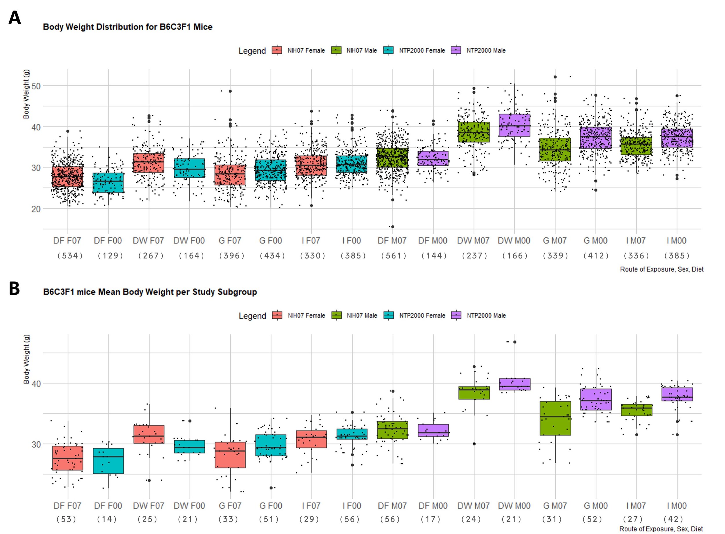
Figure 2. B6C3F1 Mouse Body Weight Distributions. Boxplots depicting the distribution of B6C3F1 mouse body weights in NTP 90-day studies according to diet consumed and route of administration of the test article. Represented in the figure by the box is the median, first quartile, third quartile, and the vertical bars represent the1.5*IQR. The IQR is calculated by finding the difference between the 25th percentile and the 75th percentile of the data (Diez et al. (2019)). The type of diet and dose route is denoted on the x-axis by DF = Dosed Feed, DW = Dosed Water, G = Gavage, I = Inhalation. F07 refers to females (F) given the NIH-07 diet, F00 refers to females given the NTP-2000 diet. Body weight (in grams) is on the y-axis. M07 refers to males (M) given the NIH-07 diet, M00 refers to males given the NTP-2000 diet.The number below the diet and dose route indicates how many data points are included in each boxplot. A. Body weight distribution of B6C3F1 mice. Female B6C3F1 mice median body weights range 26.5-31.3g and male B6C3F1 median body weights range 32.6-40.1g. B. Body weight distribution of mean body weights of B6C3F1 mice per study subgroup. The median of the male and female body weights are approximately the same as in A, but there are fewer data points exceeding the 1.5 IQR limits and the spread is generally smaller.

Figure 3. Graphical Comparison of Normally Distributed vs Non-normally Distributed Samples. A, B. Distribution of body weights from 90-day female B6C3F1 mice exposed to 1,1,1-Trichloroethane (71-55-6) via dosed feed on the NTP diet. The SW test for normality (Royston (1982)) moproduced a p-value of 0.419 and therefore, the null hypothesis of a normal distribution is not rejected. C, D. Distribution of body weights from 90-day female B6C3F1 mice exposed to 2-Hydroxy-4-methoxybenzophenone (131-57-7) via dosed feed on the NIH diet. The point in blue is a point that lies beyond the 1.5 IQR (Diez et al. (2019)). The SW test for normality produced a p-value of 0.004 and therefore the null hypothesis of a normal distribution is rejected.

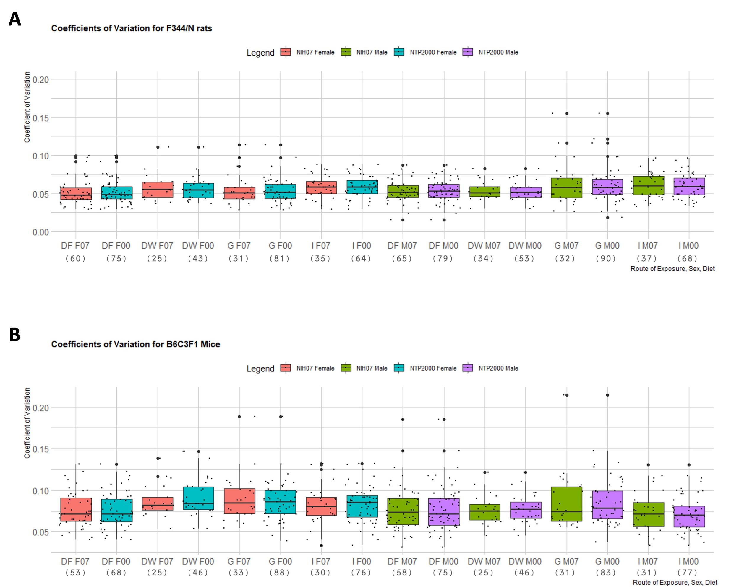
Figure 4. Distribution of the Coefficient of Variation of Each Rodent Strain. Boxplots depicting the distribution of each strain’s coefficient of variance (CVs) for terminal body weight in NTP 90-day studies according to route of administration and diet. Represented in the figure by the box is the median, first quartile, third quartile, and the vertical bars represent the 1.5*IQR. On the x-axis, the dose route is denoted by DF = Dosed Feed, DW = Dosed Water, G = Gavage, I = Inhalation. F07 refers to females given the NIH-07 diet, F00 refers to females given the NTP-2000 diet. M07 refers to males given the NIH-07 diet, M00 refers to males given the NTP-2000 diet. The y-axis shows the range of the proportion representing the CV. The number below the diet and dose route indicates how many data points are included in each boxplot. A. Distribution of CVs for F344/N rats. The IQR ranged 0.01-0.12g. B. Distribution of CVs for B6C3F1 mice. The IQR ranged 0.01-0.15g.The IQR is calculated by finding the difference between the 25th percentile and the 75th percentile of the data (Diez et al. (2019))

Table 3. Results of Testing for Normality. Proportion of rejections according to SW test with a threshold of 0.05. Proportions for F344/N rats and B6C3F1 mice were obtained by analyzing at least 25 studies per dose route. The F344/N rats showed the highest proportions of rejections across all routes of administration except for inhalation. The F344/N rats proportions of rejections ranged from <0.005%-18.46%; B6C3F1 proportions were slightly higher for the dose route inhalation with a maximum rejection proportion of 17.39% compared to F344/N rats highest proportion of rejection for this dose route being 14.29%.

	Dosed Feed		Dosed Water		Gavage		Inhalation
	F344/N	B6C3F1	F344/N	B6C3F1	F344/N	B6C3F1	F344/N	B6C3F1
1980-1994 (Female)	16.67%	7.55%	8.00%	8.00%	12.90%	12.12%	14.29%	13.33%
1980-1994 (Male)	18.46%	8.62%	14.71%	12.00%	6.25%	12.90%	5.41%	12.90%
1995-2013 (Female)	6.67%	0.00%	0.00%	19.05%	10.00%	9.09%	3.45%	17.39%
1995-2013 (Male)	7.14%	5.88%	0.00%	0.00%	1.72%	5.77%	3.23%	8.70%

Table 4. Median Skew Values of Studies Rejecting Normal Distribution. The median value of skew for studies that were rejected according to the SW test. N/A are in place where no studies were rejected according to the SW test. Skewness (g) indicate strong skew (|g| > 1), moderate skew (1 > |g| > 0.5) and very little skew (|g| < 0.5). The median ranged between -2.23 (strongly negatively skewed in Male F344/N rats in Inhalation studies in the NIH-07 diet) to 2.12 (strongly positively skewed for Female F344/N rats in Inhalation studies in the NTP 2000 diet) while the smallest |g| was 0.23 from a rejected distribution of female B6C3F1 mice via Inhalation in the NIH-07 diet (data not shown) and the largest |g|was 3.05 from a rejected distribution of male F344/N rats via Inhalation in the NIH-07 diet (data not shown).

	Dosed Feed		Dosed Water		Gavage		Inhalation
	F344/N	B6C3F1	F344/N	B6C3F1	F344/N	B6C3F1	F344/N	B6C3F1
1980-1994 (Female)	-0.70	0.91	0.43	-1.84	1.38	1.62	-1.63	0.97
1980-1994 (Male)	0.29	-0.59	-0.24	1.30	-0.37	1.77	-2.23	0.32
1995-2013 (Female)	0.32	N/A	N/A	-1.12	1.82	0.89	2.12	1.49
1995-2013 (Male)	-1.84	1.14	N/A	N/A	-1.76	1.43	1.50	1.37

False positive rate and statistical power to detect departures from normality

The false positive rate  (FPR) for the SW tests is shown in Table 5 and it can be seen that the FPR never surpassed 5.5%. Table 5 also shows the power of the SW to detect departures of normality using a skewness value of 2.87. For a  sample size of 10 rodents, there was up to 11.8% power to detect departures from normality and for a  sample size of 50 rodents there was up to 57.0% power to detect departures from normality.  

Table 5. Robustness of Shapiro-Wilk Test. The false positive rates (FPRs) and power to detect departures from normality for simulations of the SW test. FPRs were calculated with a skew (g) of 0 (no skew) and the power to detect departures from normality shown here was calculated at a skew of 2.87. The FPR never surpassed 5.5%, which is close to the typical FPR of 5.0%. For a sample size of 10 rodents, there was up to 11.8% power to detect departures from normality and for a sample size of 50 rodents there was up to 57.0% power to detect departures from normality. The level of power to detect departures from normality is consistent across all strains at each sample size. Power greater than 80% is not obtained until reaching a sample size of 100 rodents.

	False Positive Rate						Power to detect departures from normality
	F344/N   Male	F344/N   Female	HSD Male	HSD   Female	B6C3F1   Male	B6C3F1   Female	F344/N   Male	F344/N   Female	HSD Male	HSD   Female	B6C3F1   Male	B6C3F1   Female
5 Rodents	0.0453	0.0473	0.0453	0.051	0.048	0.0479	0.0669	0.066	0.0624	0.0653	0.0627	0.0633
10 Rodents	0.0453	0.0509	0.0479	0.0511	0.0508	0.0453	0.1156	0.1182	0.1142	0.1129	0.1149	0.114
20 Rodents	0.0526	0.0487	0.0473	0.0518	0.0545	0.0541	0.2298	0.2317	0.2317	0.2374	0.2281	0.2261
50 Rodents	0.05	0.0511	0.0513	0.0513	0.0504	0.053	0.5647	0.5635	0.5702	0.5626	0.5637	0.5642

False positive rate and statistical power to detect body weight differences

The FPR for both the t-test  and the Mann-Whitney test never rose above 5.1% (data not shown). The results for the power of the t test and Mann-Whitney test are found in Table 6. For a 10% difference in body weight, a skewed normal  distribution, and a sample size of 10 male F344/N rats, the t-test and Mann-Whitney test had 99.2% and  98.9% power, respectively, to detect a 10% body weight difference. Under the same conditions for male  HSD rats the t-test and Mann-Whitney test had 95.7% and 94.3% power and for male B6C3F1 mice the t test and Mann-Whitney test had 83.6% and 82.1% power, respectively, to detect a 10% body weight  difference.  

Table 6. Robustness of Parametric and Nonparametric Tests. Power of the t-test and Mann-Whitney test to detect body weight differences of 5%, 10%, and 20% for a normal distribution (γ=0) and a skew normal distribution (γ=2.87). Results from simulations of male F344/N rats, HSD rats, and B6C3F1 mice are shown. Both tests had greater than 80% to detect a 10% body weight difference from a sample size of 10 rodents for each strain. For a 10% difference in body weight, a skewed normal distribution, and a sample size of 10 male F344/N rats, the t-test and MannWhitney test had 99.2% and 98.9% power, respectively, to detect a 10% body weight difference. Under the same conditions for male HSD rats the t-test and Mann-Whitney test had 95.7% and 94.3% power and for male B6C3F1 mice the t-test and Mann-Whitney test had 83.6% and 82.1% power, respectively, to detect a 10% body weight difference.

F344/N	5% Difference		10% Difference		20% Difference
	γ=0	γ=2.87	γ=0	γ=2.87	γ=0	γ=2.87
T-Test
5 Rats	0.2952	0.3144	0.8187	0.8237	0.9997	0.9994
10 Rats	0.6089	0.6305	0.9946	0.9936	1	1
20 Rats	0.9084	0.9083	1	1	1	1
50 Rats	0.9993	0.9996	1	1	1	1
	5% Difference		10% Difference		20% Difference
	γ=0	γ=2.87	γ=0	γ=2.87	γ=0	γ=2.87
Mann Whitney
5 Rats	0.2365	0.2624	0.7354	0.7343	0.9988	0.9956
10 Rats	0.5621	0.6181	0.99	0.9902	1	1
20 Rats	0.8938	0.9168	1	0.9999	1	1
50 Rats	0.9993	0.9996	1	1	1	1
HSD	5% Difference		10% Difference		20% Difference
	γ=0	γ=2.87	γ=0	γ=2.87	γ=0	γ=2.87
T-Test
5 Rats	0.2196	0.2275	0.654	0.9718	0.9968	0.6692
10 Rats	0.454	0.4666	0.9611	1	1	0.96
20 Rats	0.7708	0.7817	0.9996	1	1	0.9997
50 Rats	0.9922	0.9941	1	1	1	1
	5% Difference		10% Difference		20% Difference
	γ=0	γ=2.87	γ=0	γ=2.87	γ=0	γ=2.87
Mann Whitney
5 Rats	0.1707	0.1842	0.5588	0.9941	0.9879	0.583
10 Rats	0.4108	0.4561	0.9427	1	1	0.9486
20 Rats	0.746	0.8036	0.9994	1	1	0.9994
50 Rats	0.9892	0.9955	1	1	1	1
B63CF1	5% Difference		10% Difference		20% Difference
	γ=0	γ=2.87	γ=0	γ=2.87	γ=0	γ=2.87
T-Test
5 Rats	0.1545	0.1501	0.4762	0.4817	0.9623	0.955
10 Rats	0.3131	0.3217	0.8373	0.8357	0.9999	0.9996
20 Rats	0.5808	0.5838	0.9893	0.9887	1	1
50 Rats	0.9319	0.9324	1	1	1	1
	5% Difference		10% Difference		20% Difference
	γ=0	γ=2.87	γ=0	γ=2.87	γ=0	γ=2.87
Mann Whitney
5 Rats	0.116	0.1191	0.3897	0.4026	0.9257	0.8988
10 Rats	0.281	0.3169	0.8007	0.8211	0.9999	0.9996
20 Rats	0.5603	0.6055	0.9845	0.9899	1	1
50 Rats	0.9167	0.9446	1	1	1	1

Bias and precision of mean body weight estimates

Statistical bias occurs when the results of a test show  differently (either overestimating or underestimating) than the true value of a parameter. The value  that we obtain for bias of the mean body weight estimate is the difference between the estimated value  of the parameter from the statistical test and the actual value of the parameter (Piedmont, 2014). For all cases examined here the average bias of the mean estimate across 10,000 simulations never exceeded 0.05% (data not shown), which is very small and makes sense given that the mean should be  an unbiased estimator of the population mean. The 95% confidence intervals for mean body weight are  presented in Table 7. The confidence intervals for a skew of 0 consistently overlaps the confidence  intervals obtained using a skew of 2.87.  

Table 7. Confidence Intervals of Parametric and Nonparametric Tests. Precision of male F344/N rats, HSD rats, and B6C3F1 mice shown by 95% confidence intervals for a normal distribution (γ=0) and a skew normal distribution (γ=2.87). The precision of the estimated parameters can be found by looking at the confidence intervals of the estimates; smaller confidence intervals are considered more precise and larger confidence intervals are less precise (Trafimow (2018)). The confidence intervals for a skew of 0 consistently overlaps the confidence intervals obtained using a skew of 2.87.

	95% Confidence Interval (γ=0)	95% Confidence Interval (γ=2.87)
F344/N Rats	Grams	Grams
5 Rats	(350.3019, 379.9536)	(351.1550, 380.7336)
10 Rats	(354.2105, 375.5990)	(355.0758, 376.0066)
20 Rats	(357.5236, 372.3938)	(357.7277, 372.6786)
50 Rats	(360.2422, 369.7929)	(360.5199, 369.8105)
	95% Confidence Interval (γ=0)	95% Confidence Interval (γ=2.87)
HSD Rats	Grams	Grams
	(418.2629, 461.4174)	(419.7195, 463.3615)
5 Rats	(424.521.16, 455.2719)	(425.3285, 456.0971)
10 Rats	(429.1162, 450.9949)	(429.5644, 451.3001)
20 Rats	(433.2238, 446.9803)	(4331.1132, 447.2053)
50 Rats	(418.2629, 461.4174)	(419.7195, 463.3615)
	95% Confidence Interval (γ=0)	95% Confidence Interval (γ=2.87)
B6C3F1 Mice	Grams	Grams
5 Mice	(32.86719, 37.15108)	(32.95023, 37.36299)
10 Mice	(33.42615, 36.55389)	(33.54174, 36.64461)
20 Mice	(33.90853, 36.08742)	(33.96725, 36.12804)
50 Mice	(34.31297, 35.70167)	(34.32235, 35.70336)

DISCUSSION

Observation of the median body weights for each strain in Figures 1A and 2A shows that the mouse  body weights are more variable than F344/N rat body weights. Hoffman et al. (2002) has also reported  that mouse body weights are usually more variable than rat body weights. This appears to be true for  the data presented in this analysis according to Figure 4. It can be seen from Figures 1 and 2 that in  each species males weigh more than females and there are different levels of variability in each dose  route group. While the F344/N rats tend to have similar median body weight across all dose routes with  respect to sex, B6C3F1 mice have more variable median body weights across all dose routes. It is  interesting to note that Figures 1A also shows median body weights, in general, appear slightly higher  for rats consuming NIH-07 diet compared to NTP-2000. In contrast, Figure 2A shows that median body  weights, in general, appear slightly higher for mice consuming the NTP-2000 diet. Another factor that  must be considered is the variability of the number of animals in each dose route group. For 90-day  dosed feed studies a total of 638 F344/N male rats and 660 B6C3F1 male mice were included. For  dosed water studies a total of 320 F344/N males and 308 B6C3F1 males were included. These  imbalances are reflected in the gavage and inhalation dose route groups as well. In addition, rats fed  NTP 2000 diet tended to have lower median body weights than rats fed NIH-07 diet as seen in Figure 1.  When looking at Figure 2, both the median of observed body weights (Figure 2A) and the median of the  mean body weight of each subgroup appear to be higher for B6C3F1 mice fed the NTP-2000 diet rather  than the NIH-07 diet. This difference in body weight was shown to be statistically significant through a  Mann-Whitney test comparing the body weights of rodents fed the NIH-07 diet and rodents fed the  NTP-2000 diet (data not shown).  

Although we examined several different normality tests (data not shown), the Shapiro-Wilk test has  been widely used and is accepted as a powerful statistical test for normality (Ghasemi & Zahediasl,  2012). Through the simulations performed with the Shapiro-Wilk test to detect departures from  normality, a larger sample size of 50 rodents only showed up to 57% power, far below the 80% power  that is desired of most applications of statistical tests (Cohen, 1988). In Cohen’s Statistical Power  Analysis for the Behavioral Sciences (1988), the author demonstrates that due to the funds and  resources needed for most experiments to obtain the sample sizes generally used, 80% power is the  conventional rule of thumb that researchers should strive to obtain or attain. Therefore, we  implemented the Shapiro Wilk test for normality in unison with graphical methods to assess normality in  this study.  

The t-test was highly robust to departures from normality in the simulation studies of the 90-day data.  An approximate 10% or greater body weight difference between control and treated groups indicates  adverse effects (World Health Organization, 2009). This is consistent with the findings of Sullivan and  D’Agostino (1992). That study investigated the difference in power from a t-test performed with  skewed data and power from a t-test performed with simulated data following a normal distribution and  found differences were very small. The same can be seen in the results; the power to detect a 10%  difference in body weights compared to controls from skew normal distributions and the power to  detect a 10% difference in normally distributed body weights compared to controls with a sample size of  10 are within 2% of each other. For a skew normal distribution and a sample size of 10, the t-test had at  least 80% power to detect a 10% body weight difference. From Table 6 the t-test showed false positive  rates (FPR) of simulated data with no skew only rose above 5% for B6C3F1 mice in groups of 10 (FPR of  5.07%), HSD rats in groups of 20 (FPR of 5.15%), and HSD rats in groups of 50 (FPR of 5.40%). When data with a skew normal distribution was simulated, the t-test showed false positive rates rose above 5% for  F344/N rats in groups of 50 (FPR of 5.22%) and B6C3F1 mice in groups of 50 (FPR of 5.38%). The Mann Whitney test showed false positive rates of simulated data with no skew only rose above 5% for HSD  rats in groups of 50 (FPR of 5.31%). For skew normal data, the Mann-Whitney test showed false positive  rates above 5% for B6C3F1 mice in groups of 50 (FPR of 5.01%). 

The diet used in NTP studies changed in 1994 to reduce the protein-to-fat ratio, aiming to keep  laboratory rodents healthier as they aged. The NIH-07 (1980-1994) diet was 24% protein, 5% fat, and  3.5% fiber and the NTP-2000 (1995-present) diet is 14.5% protein, 8.5% fat, and 9.5% fiber (Rao, 1996).  The NTP-2000 diet showed evidence of decreased lesions in F344/N rats compared to rats fed the NIH 07 diet (Rao, 1996). The results show in some cases there is an increase in the percentage of rejections  of normality for studies using NTP-2000 diet for F344/N rats and B6C3F1 mice. A possible reason that  there may be an increase in departures from normality using the NTP-2000 diet compared to the NIH-07  diet is that the F344/N strain was highly inbred and began to show an increase in leukemia and other  types of tumor (King-Herbert et al., 2010) that could influence body weight. In fact, this circumstance  motivated the NTP to make the switch to using the Harlan Sprague-Dawley strain as their primary rat  strain in studies (King-Herbert et al., 2010). As mentioned earlier, a minimum of 25 studies for F334/N  and B6C3F1 were used in the analysis shown in Table 3 but a maximum of 90 F344/N rat studies was  obtained as well as a maximum of 88 B6C3F1 mouse studies. The number of studies available to us with  HSD rat data was much more limited, with a minimum of 2 studies in the dosed water dose route and a  maximum of 23 studies in the gavage dose route. HSD rats were not included in this portion of the  analysis due to this reason. 

Overall, data from 90-day studies showed little deviation from normality while the HSD strain showed  no deviation from normality. Rao and Crockett (2003) suggest that choice of diet and housing type for  B6C3F1 mice greatly impact the mortality rates and tumor growth of these mice. This gives a possible explanation for the different levels of variation between the different diets and dose routes. Both the t test and Mann-Whitney test show 80% power to detect a 10% body weight difference at various  distributions. Based on our simulation results, large enough sample sizes allow our parametric tests to  handle populations that do not follow a strict normal distribution. In this case, a sample size of 10 was  sufficient in order for the t-test to have adequate power and control the false positive rate at  approximately 5%.  

Discoveries and challenges from the analysis of body weights

Our approach to this study assessed if  parametric testing could have adequate power and accuracy to test differences between two groups  that have a skew normal distribution. Due to parametric tests relying on an approximately normal  distribution, the investigation of a skew normal distribution both adhered to an approximately normal  distribution while also investigating the effect of deviations from normality on parametric testing. This  analysis provided us with insight as to how certain design variables may affect body weight differences  between groups. Haseman et al. (1994) found that individually housed B6C3F1 male mice showed a  decrease in the development of certain tumors and an increase in survival compared to those housed in  groups. It has been observed when rodents are housed together, there is often a decrease in food  consumption by certain members of the group causing variable weight gain/loss within the group  (Gonder & Laber, 2007). On the other hand, group housing has shown that rodents are able to adapt  better to stress rather than when individually housed impacting weight along with many other factors  (Gonder & Laber, 2007). A study by de Torrente et al. (2019) explores how the shape of the distribution  considered in a statistical test affects the outcome. Once they began using the distribution information  for each data set, they were able to improve the survival predictions of cancer patients. This  corresponds to studies that showed multimodality of rodent body weights but did not consist of  different control groups. Similar to how we looked at different levels of skewness of the skew normal  distribution, a deeper look into body weight distribution may alter the outcome of which statistical tests should be used when evaluating those studies. A study by Razali & Wah (2011) compared the power of  the SW test, Komogorov-Smirnov, Lilliefors, and Anderson-Darling tests to detect departures from  normality from simulated data. They found that the SW test is the most powerful of the four tests for  detecting departures from normality, strengthening our usage of the SW test to test for normality testing. Not only is an investigation of the distribution of rodent body weight data important, but it is  important to understand the distribution of any endpoint of interest. A review by Mar (2019) discusses  the importance of distributional assumptions in the field of genetics (specifically studying gene  expression and regulation) it is imperative to understand the distribution of the data being tested in  order to obtain the most accurate statistical results; even with large data sets. Another example of data  distribution being studied in gene expression is a study by Church et al. (2019). This study sought to  understand different distributions common in certain patient cohorts, further motivating our  exploration of non-normality of each species/strain/sex/dose route. 

We did not remove potential outliers or influential observations in this study. However, removal of  statistical outliers could change the results of normality tests. There is debate on how and when to  remove statistical outliers. The removal of statistical outliers without justified cause could make a dataset appear more normal than it is and mask its true distribution (Millard, 2019). The removal of outliers according to Tukey’s Outer Fences (Tukey, 1977) shows up to 10% decrease in proportion of  rejections of the 90-day studies and up to 40% decrease in chronic 2-year studies (data not shown). This  is supported by the findings of Frecka and Hopwood (1993). That study found that the inclusion of  outliers changed the parameter estimations for the distributions of their data. Once outliers were  removed, normal distributions were seen for the same data. On the other hand, Osborne and Overbay  (2004) also argues that the removal of extreme outliers is beneficial to the statistical analysis of data,  especially when using parametric tests. Osborne and Overbay came to this conclusion after performing  multiple simulations with t-tests and ANOVA where they compared false positive rates and false negative rates before and after the removal of outliers. The accuracy of the mean estimates was also  improved upon the removal of outliers in their study. 

Looking at Chronic Study Body Weight Measurements

This analysis also included a brief look into the  distribution of chronic (2-year) study terminal body weight measurements by the same methods used  for analysis of the 90-day study data, but results are not shown. Chronic study data showed more  departures from normality than 90-day data. Simulations for parametric and nonparametric testing  revealed that the tests held at least 90% power to detect 10% difference in terminal body weight for a  sample size of 25 for F344/N male rats but held less than 55% power to detect a 10% difference in  terminal body weight for a sample size of 25 HSD male rats and less than 20% power to detect a 10%  difference in terminal body weight for a sample size of 25 for B6C3F1 male mice. A decrease in sample  size due to mortality of rodents throughout chronic studies could potentially increase the number of  distributions that deviate from normality in the dataset at a 2-year time point due to increased presence  of disease or death in aging animals. In a technical report of a study involving B6C3F1 mice and  exposure to Oxazepam, a 65-75% survival rate was seen at 2 years, which is typical for the terminal  sample sizes in the dataset obtained (National Toxicology Program, 1993).  

Future Directions

Similar to the normality assumption, many parametric tests assume there is equal  variance across the data groups (Garson, 2012). In addition, regarding the chronic study data, looking at  interim body weight measurements, such as at six months or one year, would give insight on the  distribution of the rodents’ body weights throughout the study and would increase the sample size at  certain time points allowing an investigation of how variability changes over time. A further endpoint  for which to evaluate normality is organ weight, another key variable measured in toxicology studies for  which normality is often assumed. While we used the skew normal distribution to model departures  from normality, future studies could explore the consequences of stronger departures from normality. Since we have investigated the normal assumption, it would also be beneficial to investigate the equal variance assumption across dose groups for body weight data. It would also be beneficial to explore  whether body weight differences are associated with design variables such as housing, diets, etc. As  mentioned in the discussion, housing and diet can play a crucial role in the distribution of laboratory  rodent body weight measurements.  

ACKNOWLEDGEMENTS 

This research was supported [in part] by the Intramural Research Program of the National Institutes of  Health (NIH), National Institute of Environmental Health Sciences (NIEHS). We thank Laura Betz (Social &  Scientific Systems) and Dr. Pei-Li Yao (Program Operation Branch, NTP) for reviewing the manuscript and  providing helpful suggestions.

REFERENCES

1. Abdi, H. (2010). Coefficient of variation. Encyclopedia of research design, 3, 170-170.
2. Azzalini, A. (2011). Skew-Normal Distribution. In L. M. (Ed.), International Encyclopedia of Statistical Science.,. Springer.
3. Azzalini, A. (2019). The R package ’sn’: The Skew-Normal and Related Distributions such as the Skew-t (version 1.5-4).,. Retrieved from http:// azzalini.stat.unipd.it/SN
4. Bauer, D. F. (1972). Constructing confidence sets using rank statistics. Journal of the American Statistical.
5. Chhabra, R. S., Huff, J. E., Schwetz, B. S. and Selkirk, J. (1990). An overview of prechronic and chronic toxicity/carcinogenicity experimental study designs and criteria used by the National Toxicology Program. Environmental Health Perspective, 86, 313-321.
6. Church, B. V., Williams, H. T. and Mar, J. C. (2019). Investigating skewness to understand gene expression heterogeneity in large patient cohorts. BMC Bioinformatics(24), 20-20.
7. Cohen, J. (1988). Statistical Power Analysis for the Behavioral Sciences,.
8. Curran-Everett, D. (2017). Explorations in statistics: The assumption of normality. Advances in Physiology Education, 41(3), 449-453.
9. Diez, D., Cetinkaya-Rundal, M. and Barr, C. D. (2019). OpenIntro Statistics.,. OpenIntro.
10. Frank, S. A. (2009). The Common Patterns of Nature. Journal of Evolutionary Biology, 22(8), 1563-1585.
11. Frecka, T. J., and Hopwood, W. S. (1983). The Effects of Outliers on the Cross-Sectional Distributional Properties of Financial Ratios. The Accounting Review, 58(1), 115-128.
12. Garson, G. D. (2012). Testing Statistical Assumptions. Blue Book Series. . Statistical Associates Publishing.
13. Ghasemi, A., and Zahediasl, S. (2012). Normality Tests for Statistical Analysis: A Guide for Non-Statisticians. International Journal of Endocrinology and Metabolism, 10(2), 486-489.
14. Gonder, J. C., and Laber, K. (2007). A Renewed Look at Laboratory Rodent Housing and Management. ILAR Journal, 49(1), 29-36.
15. Haseman, J. K., Bourbina, J. and Eustis, S. L. (1994). Effect of Individual Housing and Other Experimental Design Factors on Tumor Incidence in B6C3F1 Mice. Fundamental and Applied Toxicology, 23(1), 44-52.
16. Hayes, A. W., and Kruger, C. L. (2014). Hayes’ Principles and Methods of Toxicology. London: CRC Press.
17. Hermanussen, M., Danker-Hopfe, H. and Weber, G. W. (2001). Body weight and the shape of the natural distribution of weight, in very large samples of German, Austrian and Norwegian conscripts. International Journal of Obesity and Related Metabolic Disorders, 25(10).
18. Hoffman, W. P., Ness, D. K. and Lier, R. B. L. V. (2002). Analysis of Rodent Growth Data in Toxicology Studies. Toxicological Sciences, 66(2), 313- 319.
19. John, J. M. M., Lishout, F. V., Gusareva, E. S. and Steen, K. V. (2013). A robustness study of parametric and non-parametric tests in modelbased multifactor dimensionality reduction for epistasis detection. BioData Mining, 6(9).
20. Kim, J. H. T. (2010). Bias correction for estimated distortion risk measure using the bootstrap. Insurance: Mathematics and Economics, 47, 198- 205.
21. King-Herbert, A. P., Sills, R. C. and Bucher, J. R. (2010). Commentary: Update on Animal Models for NTP Studies. Toxicologic Pathology, 38(1), 180-181.
22. Lea, I. A., Gong, H., Paleja, A., Rashid, A. and Fostel, J. (2016). CEBS: A comprehensive annotated database of toxicological data. Nucleic Acids Research, 45(D1).
23. Lewis, R. W., Billington, R., Debryune, E., Gamer, A., Lang, B. and Carpanini, F. (2002). Recognition of Adverse and Nonadverse Effects in Toxicity Studies. Society of Toxicologic Pathology, 30(1), 66-74.
24. Lumley, T., Diehr, P., Emerson, S. and Chen, L. (2002). The Importance of the Normality Assumption in Large Public Health Data Sets. Annual Review of Public Health, 23(1), 151-169.
25. Mar, J. C. (2019). The rise of distributions: why non-normality is important for understanding the transcriptome and beyond. Biophysical Reviews, 11, 89-94.
26. Maronpot, R. R., Nyska, A., Foreman, J. E. and Ramot, Y. (2016). The legacy of the F344 rat as a cancer bioassay model (a retrospective summary of three common F344 rat neoplasms). Critical Reviews in Toxicology, 46(8), 641-675.
27. Mcgill, R., Tukey, J. W. and Larsen, W. A. (1978). Variations of Box Plots. The American Statistician, 32(1), 12-16.
28. Meyer, D., Dimitriadou, E., Hornik, K., Weingessel, A., Leisch, F., Chang, C. and Lin, C. (2019). Package ‘e1071’: Mic Functions of the Department of Statistics, Probability Theory Group (version 1.7-4).,. Retrieved from http://sunsite2.icm.edu.pl/pub/unix/math/cran/web/packages/e1071/e1071.pdf 
29. Millard, S. P. (2019). EPA is Mandating the Normal Distribution. Statistics and Public Policy, 6(1), 36-43.
30. Moore, D. S., and Mccabe, G. P. (2001). Introduction to the Practice of Statistics,. New York, NY: W. H. Freeman and Company.
31. NTP Technical Report on the Toxicology and Carcinogenesis. Studies of Oxazepam (CAS No. 604-75-1) in Swiss-Webster and B6C3F1 Mice (feed studies)., (1993). Retrieved from https://ntp.niehs.nih.gov/ntp/ htdocs/lt_rpts/tr443.pdf 
32. Organization, W. H. (2009). Toxicological and Clinical Studies and Evaluation for Hazard Identification and Characterization in Principles and methods for the risk assessment of chemicals in food. Geneva: World Health Organization, 4, 1-4.
33. Osborne, J. W., and Overbay, A. (2004). The Power of Outliers (and Why Researchers Should Always Check for Them). Practical Assessment, Research, and Evaluation, 9(6), 1-8.
34. Piedmont, R. L. (2014). Bias, Statistical. In M. A.C. (Ed.), Encyclopedia of Quality of Life and Well Being Research.,. Dordrecht: Springer.
35. Rao, G. N., and Crockett, P. W. (2003). Effect of Diet and Housing on Growth, Body Weight, Survival and Tumor Incidences of B6C3F1 Mice in Chronic Studies. Toxicologic Pathology, 31(2), 243-250.
36. Rasch, D., and Guiard, V. (2004). The robustness of parametric statistical methods. Psychology Science, 46(2), 175-208.
37. Razali, N., and Wah, Y. B. (2011). Power comparisons of Shapiro-Wilk, Kolmogorov-Smirnov, Lilliefors and Anderson-Darling tests. Journal of Statistical Modeling and Analytics, 2(1), 21-33.
38. Rochon, J., Gondan, M. and Kieser, M. (2012). To test or not to test: Preliminary assessment of normality when comparing two independent samples. BMC Medical Research Methodology, 12(1).
39. Royston, P. (1982). An extension of Shapiro and Wilk’s W test for normality to large samples. Applied Statistics, 31(2), 115-124.
40. Shockley, K. R., and Kissling, G. E. (2018). Statistical Guidance for Reviewers of Toxicologic Pathology. Toxicology Pathology, 46(6), 647- 652.
41. Statistical Procedures., (2018). Retrieved from https://ntp.niehs.nih.gov/ testing/types/stats/index.html 
42. Sullivan, L., and D’Agostino, R. (1992). Robustness of the t Test Applied to Data Distorted from Normality by Floor Effects. Journal of Dental Research, 71(12), 1938-1943.
43. Torrenté, L. D., Zimmerman, S., Suzuki, M., Christopeit, M., Greally, J. M. and Mar, J. C. (2019). The shape of gene expression distributions matter: How incorporating distribution shape improves the interpretation of cancer transcriptomic data. BioRXiv.
44. Trafimow, D. (2018). Confidence intervals, precision and confounding. New Ideas in Psychology, 50, 48-53.