

UTTAM BHETUWAL, ANGEL CHAVEZ, ISAAC DOBES
Carnegie Mellon University, 5000 Forbes Avenue, Pittsburgh, PA 15213, USA
ABSTRACT
This paper focuses on minimal risk strategies for tournament style No-Limit Texas Hold’em. In order to obtain the most favourable outcome, we write linear programs which provide a set of constraints for a conservative player to follow so that a favorable outcome is obtained. We also model strategies by constructing stack functions, which map a strategy to its expected outcome. We prove various properties of stack functions, which provide evidence in support of the conjecture that the minimal risk strategy corresponds to the line segment connecting (0, yo) to (n, A), where yo is the initial number of chips a player has in the tournament, and A is the desired amount of chips a player has at the end of the tournament.
INTRODUCTION
The game of poker is exciting for many and offers the potential for monetary gain. Nonetheless, the risk of losing large quantities of money deters many from taking part in the game. To mitigate risk, we analyze and model minimal risk strategies.
In this section, we first describe the rules of No-Limit Texas Hold’em (NLTH) and its implications in a tournament setting. Then we define risk and conservative play, and characterize the Zero Risk strategy.
After defining the Zero Risk strategy, we formulate the linear programs which provide a guideline for a player attempting to minimize risk. We then take a more theoretical approach and use various metrics to measure components of risk: aggressiveness, C1 norms, and total variation.
The Rules of NLTH
No-Limit Texas Hold’em poker is an n player (2 ≤ n ≤ 10) game of incomplete information, that uses the standard 52 card playing deck. At the beginning of a hand, each player is dealt two cards. Player only have knowledge of cards dealt to them.
Once the players are dealt their two cards, two players are required to place bets, called the small blind and big blind bets. The big blind is always twice the amount of the small blind. Both blinds rotate around the table to different players after each hand to ensure all players will eventually be place a small and big blind. Once the big blind bets, a round of betting begins: players must either (1) call meaning they bet an equal number of chips as the player before them, (2) raise meaning they bet more chips then the player before them, (3) fold meaning they do not bet any chips and forfeit out of the hand, they also lose any chips they have bet in the hand, or (4) check meaning they defer the decision to call, bet, or fold, a decision must be made eventually. A round of betting is complete once every player calls, and no player desires to raise. Note that for the small blind to continue playing must also call or raise the big blind (or subsequent raises of the big blind); if they fold, then they lose the small blind they were forced to bet in the beginning. After this round of betting is complete, three community cards are placed face up on the table and similar rounds of betting proceed. After the rounds of betting are complete, the player with the best five card hand then wins the pot, which is the accumulation of all chips bet from the beginning of the hand. The best five card hand (two personal cards and three community cards) is determined by the usual poker rules.
NLTH Tournament Rules
In a NLTH tournament, many (sometimes over a thousand) players at different tables of nine each start with the same amount of chips and continuously play hands until they either run out or are the last player remaining, in which case they win the tournament and accept a cash prize. To facilitate betting and hasten the game, blind bets increase after a certain period of time. The period of time in which the blinds are a fixed amount is called a level, when the time period is over the players move into a new level and the blinds increase. In the beginning of the tournament, after a certain number of levels, an ante bet is introduced The ante bet requires that all players bet a specified number of chips at the beginning of every hand; the blind bets still apply. The ante bets never decrease after a level, and like the blind bets, can and often increases after a level.
Risk and Conservative Strategies
Definition 1
Risk per hand is defined as the probability of losing the hand multiplied by the value bet in the hand. For a given hand i, the risk of hand i is denoted by r(i).
Remark: The blind and ante amounts are not accounted for in this definition of risk; since they are mandatory bets they are considered sunk costs.
Definition 2
A strategy is a sequence of decisions allowable to a player in the game. The overall risk of a strategy is the expected value of the risk of the strategy, given by

where N denotes the total number of hands played in the duration of the strategy.
Definition 3
A conservative strategy is a strategy which attempts to minimize risk.
The Zero Risk Strategy
In the Zero Risk strategy, a player checks when possible, and folds otherwise. The only time a player bets chips is when they are a blind, or if an ante bet is required by all players. Since blind and ante bets are sunk costs, in this strategy, a player voluntarily bets exactly 0 chips, incurring a risk of 0 for every hand; hence the name.
THE LOSS FUNCTION
In this section, we derive the loss function, which calculates how many chips a player will have at the end of a level, n, utilizing the Zero Risk strategy.
First Order Linear Difference Equations
To derive the loss function, we use the following theorem. The proof of the theorem can be found in Jensen (2011).
Theorem 4
Let an and dn, n ϵ N0, be real valued sequences. Then the linear first order difference equation
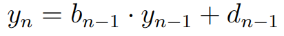
with initial value y0 ϵ R has the unique solution

Derivation of Loss Function
Since we assume that we lose every hand we bet and we only bet the required amount via blind and ante, we can use the following recursive equation to find the number of chips left at the end of level n:

where h is the number of hands played in a level (this is assumed to be a constant), an is the ante amount in level n, sn is the small blind amount in level n (note that for any level n, the big blind amount in level n is twice the small blind amount in level n), fsn is the small blind frequency in level n (that is, how many times we are the small blind), and fbn is the big blind frequency in level n (that is, how many times we are the big blind). The terms on the right hand side of the equation, excluding yn−1, make up the term cn−1 in the recursive function in Theorem 4.
Applying Theorem 4, we have the formula:

where ck = h · ak + fsk · sk + 2 · fbk · sk. Note that this formula calculates the amount of chips left at the end of level n by subtracting the cost of the n levels from the initial amount of chips a player begins with.
Position and Blind Frequency
Definition 5
For any n ϵ N, φn := initial position in level n with respect to the small blind.
That is, if a player has φn = 0, this means that they start level n as the small blind; if a player has φn = k, k ϵ [1, . . . , 8], then they are k hands dealt away from being the small blind.
Remark: If a player is currently the small blind, then they will be the big blind in the next hand. The player who is the big blind is now 8 hands away from being the small blind again.
Proposition 6
φn = φ1 − (n − 1)r (mod 9)
Proof: To prove the proposition, we use induction on the level n.
Base Case (n = 1): φ1 = φ1 − (1 − 1) · r (mod 9).
Induction Hypothesis: Suppose that for k ϵ Z, φk = φ1 − (k − 1)r (mod 9).
Induction Step: When n = k + 1,
φ1 − kr (mod 9) = φ1 − [(k − 1) + 1]r (mod 9)
= φ1 − (k − 1)r + r (mod 9)
= φk + r (mod 9), by the induction hypothesis
= φk + 1 (mod 9)
By division algorithm h = 9q + r, for some q, r ϵ Z with 0 ≤ r ≤ 9. This indicates that position, from one level to the next, is solely determined by the remainder.
Proposition 7
Let r = h (mod 9), φ1 be a player’s initial position at the beginning of the tournament, and φn be the player’s initial position at the beginning of level n. Then the following are true:
1. if φn < r, then fsn = [h/9], otherwise fsn = [h/9]
2. if φn < 8 + r (mod 9) or φn = 8, then fbn = [h/9]
Proof:
1. Consider the case where 9 is a divisor of h. Then there exists k ϵ N such that h = 9k which implies that r = 0. It is clear that each player is the small blind k =h/9 = [h/9] = [h/9] many times.
If 9 is not a divisor of h, then by the division algorithm, h = 9k + r, 0 < r < 9. 9k hands are played and thus every player is the small blind k times. After the 9kth hand, r hands remain to be played. The player with φn = 0 and the players with φn ≤ r − 1 will have the opportunity to be the small blind once more; they are the small blind k + 1, or equivalently [h/9], many times. Players with φn > r − 1 will not be able to play as the small blind again in the level; they are the small blind a total of k or [h/9] times.
2. Consider the case where 9 is a divisor of h. Then there exists k ϵ N such that h = 9k, which implies that r = 0. Therefore every player will play each position (including position 8) exactly k = h/9 = [h/9] = [h/9] times.
If 9 is not a divisor of h, then by the division algorithm, let h = 9k + r, 0 < r < 8. 9k hands are played and thus every player is the big blind k times. After the 9kth hand, r hands remain to be played. The player who started as position 8 will be the big blind again after 9k hands, so the player with φn = 8 will be the big blind k + 1 or [h/9] times. Now there are r − 1 remaining hands to be played in the level. For players that started with initial positions r − 1 or fewer hands away from the big blind, they will also be the big blind k + 1 or [h/9] times. By definition of position, these are players with initial position φn < r − 1 = 8 + r (mod 9). All of the other players won’t have the chance to become big blind again. As a result, they only get to be big blind k = [h/9] times.
Since the number of hands per level, h, is a constant, in conjunction with Proposition 7, the only input for the function required by the user is the betting structure, which in practice will be known to the player prior to entering the tournament. Therefore, if a player is utilizing the Zero Risk strategy in a tournament, they can use our function to determine how long they will last in the tournament.
INTEGER LINEAR PROGRAM (ILP)
While minimizing risk to zero may sound optimal, this notion is refuted in practice. In reality, a player utilizing the Zero Risk Strategy will often last only a few levels (about 5-7 using the World Series of Poker betting structure). This is why it is necessary to introduce risk and voluntary betting. Nonetheless, a player may still want to minimize risk subject to the following constraint: survive to the level n with at least A chips, n, A ϵ N. We refer to such a constraint as a survival constraint. We have tried and tested different iterations of ILP to get a minimal risk betting strategy.
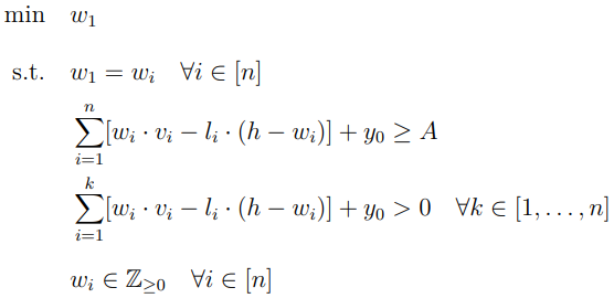
Minimum Hand ILP
To satisfy the survival constraint, one method we have developed is to minimize the number of hands played in a tournament. Let wi be the number of hands a player wins in level i, vi be the minimum value of winning a hand in level i (vi = 9 · ai + 3 · si, as each player is required to bet the ante and the big blind is twice the small blind), and li be the 8 amount of chips lost in a hand in level i:
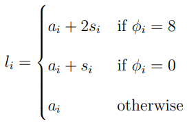
For programming purposes, we approximate li to be ai + 1/3si. We therefore formulate the Minimum Hand ILP as follows:

Note that the survival constraint for this LP is given in lines 2 and 3. In subsequent linear programs, the LP’s survival constraint to these two lines. Also, the vector w ϵ Zn consisting of the components wi, 1 ≤ i ≤ n, is a solution vector if it satisfies the survival constraints.
Issues with the Minimum Hand ILP
Due to the betting structure of tournaments, winning a hand in a later level results in a greater payoff than winning a hand in an earlier level. Therefore, to minimize the required number of hands won in n levels subject to the survival constraint, the above ILP will dictate that a player wins most of the hands in the latter levels, clustering these hands in "close" proximity. This is problematic because playing with greater frequency gives more information to other players. This decreases the players’ probability of winning the hand, thus increases the overall risk. Furthermore, requiring a player to play hands in close proximity limits what hands the player can choose to play, potentially forcing the player to play worse hands, thereby reducing their probability of winning the hand, which increases risk. Since the Minimum Hand ILP clusters the required hands won in later levels and does not require the player to win hands in earlier levels, the player is in a later level and forced to win all hands played. They may not have enough chips to bet and call opponents, making it difficult if not impossible to satisfy the survival constraints.
Uniformly Distributed ILP
To prevent clustering of required hands won, we develop another integer linear program which determines the smallest number of required hands won for a level w*, so that if exactly w* hands are won each level, then a player would satisfy the survival constraints. We call the value w*/h the minimum ratio, since it is the ratio of the smallest number of required hands won per level to the number of hands dealt in a level. We formulate below what we refer to as the Uniformly Distributed Linear Program (UDLP), which we claim (and later prove) solves the problem of finding w*.
Minimum Ratio Proposition
Since wi = w1 for all i ϵ [n], this LP has the corresponding solution vector w ϵ Zn with each component having the same value.
Proposition 8
Given the survival constraints for n levels in a tournament, the UDLP returns w*.
Proof: Suppose the UDLP has the corresponding solution vector w ϵ Zn, where each component has the value w1 ϵ Z. Assume for the sake of contradiction that there exists a solution vector v ϵ Zn, such that max1≤i≤n vi < w1. Let ṽ ϵ Zn be the vector with every 1≤i≤n component having the value max1≤i≤n vi. This satisfies all of the constraints in the UDLP, which contradicts the objective of the UDLP, since w1 is not minimal.
Minimum Ratio ILP
Let the corresponding solution vector to the UDLP be w ϵ Zn, with each component having the value w*. There may exist a solution vector satisfying the survival constraints and having maximum (component-wise) value w*, while having other components with smaller values. Below we formulate an integer linear program whose solution corresponds to the solution vector consisting of the smallest of such components.

Notice the similarities between the Minimum Ratio ILP and the Minimum Hand ILP. Because of the objective of the LP and the constraint wi ≤ w* for all i, we reduce clustering in latter levels, which is the primary defect of the minimum hand LP. Furthermore, since the Minimum Ratio ILP has an upper bound on the number of hands a player can win in a level, it requires that the player win hands in earlier levels, which prevents the player’s chips stack from falling too close to zero. This ensures that the player will have sufficient chips to place bets in latter levels.
Example
To illustrate the deficiencies of the Minimum Hand ILP and the superiority of the Minimum Ratio ILP, we ran an example. We attempted to use realistic numbers in our example, with an initial chip amount of yo = 25000 and a desired ending chip amount of A = 100000. We wanted to last 8 levels with 63 hands per level. The betting structure of this example is as follows: antes are ai = 0 if i ≤ 3 else 25 · 2i−2, blinds are si = 10 · 2i−2. With this information we ran the Minimum Hand ILP which returned

Running the UDLP gave w* = 15. We then ran the Minimum Ratio ILP, which returned

Notice that there is a greater clustering of hands in the later levels in the Minimum Hand ILP. Even though the Minimum Ratio ILP requires that we win more hands, since these 12 hands are more evenly distributed throughout all levels, we do not risk having our chip stack falling too close to zero and not being able to survive later levels.
Consider the chip stack of a player following the Minimum Hand ILP strategy it is straight forward to show the chip stack at the end of the levels is (0, 25000), (1, 24811), (2, 24370), (3, 23551), (4, 15550), (5, 2144), (6, 605), (7, 7717), and (8, 102953). We can graph this data.

Figure 1.
Consider the chip stack of a player following the Minimum Hand ILP strategy. It is straight forward to show the chip stack at the end of the levels is (0, 25000), (1, 24811), (2, 24370), (3, 23551), (4, 15550), (5, 4677), (6, 18339), (7, 45717), and (8, 100419). We can graph this data.

Figure 2.
STACK FUNCTIONS
Recall that a strategy is a sequence of decisions. Here, a strategy is defined on the number of hands, nh, in a tournament (there are h hands per level, and n levels). Therefore, a strategy is a sequence of betting decisions per hand. At each hand, the outcome of the hand is a random variable X: Ω → Z defined by ω |→ α, where ω ϵ Ω is a point in the sample space of possible betting amounts, and α is the amount a player has left at the end of the hand. The outcome of a strategy is the stochastic process {Xt : t ϵ [nh]}; that is, the outcome of the strategy is the sequence of random variables mapping the outcome of a given hand to a chip amount. The expected outcome of a strategy S, E(S) is the sequence {E(Xt) : t ϵ [nh]}, where E is the expected value operator. The discrete stack function maps a strategy to its expected outcome. Hence, a discrete stack function will return a set of nh points corresponding to expected chip amounts at given hands based on the decisions made in the strategy.
Polynomial Interpolation
Given a discrete stack function S defined on n levels (and therefore nh hands), we use Lagrange Interpolation to construct a smooth curve that best fits the outputs of the discrete function.
Theorem 9
MAT 772 (2011); Mayers and Suli (2003) Let x0, x1, ..., xn be n + 1 distinct numbers, and let f(x) be a function defined on a domain containing these numbers. Then the polynomial defined by

is the unique polynomial of degree n that satisfies pn(xj) = f(xj), j = 0, 1, ..., n, where

The polynomial pn(x) is called the interpolating polynomial of f(x).
Given a strategy S with the corresponding discrete stack function S1, we construct the strategy’s continuous stack function S2 by applying the above theorem. As we consider hand 0 to be the beginning of the tournament where every player has y0 many chips, we define f(x) on [0, . . . , nh] and f(x) = S1. Since continuous stack functions are polynomials, they are continuously differentiable on their domain [0, nh] ⊆ R. The function space C1([0, nh]) is the set of all continuously differentiable functions defined on [0, nh] ⊆ R. Hence it contains all continuous stack functions under consideration.
Aggressiveness
Definition 10
Tao (2008) The function space C1([0, nh]) is equipped with the C1 norm
||f||C1∞([0,nh]) := ||f||L∞([0,nh]) + ||f'||L∞([0,nh])
where ||f||L∞([0,nh]) := sup{|f(x)| : x ϵ [0, nh]} is the supremum norm.
The norm measures the magnitude of a stack function and the magnitude of its derivative. The magnitude of a stack function’s derivative is called the aggressiveness of a stack function. It measures the maximum magnitude of chips a player bet and won or bet and lost in a tournament.
Theorem 11
The stack function characterized by the line segment y0A is the continuous stack function which minimizes aggressiveness among all stack functions satisfying the survival constraints. We make the assumption that such this stack function exists since we are trying to determine the ideal, not necessarily practical, minimal risk strategy.
Proof: Let S be a stack function which exactly meets the survival constraints. Let yoA be the line segment connecting yo to A. By the Mean Value Theorem, there exists z in the domain of S such that S'(z) = A−yo / n−0. If S(z) ∉ yoA, then there exists ε > 0 such that

Hence, maxxϵdom(S) {|S'(x)|} > | A−yo / n−0 |. Therefore, y0A minimizes aggressiveness among all possible strategies which exactly meet the survival constraints.
Corollary 12
The stack function characterized by the line segment y0A is the continuous stack function which minimizes the C1 norm of all stack functions which exactly meet the survival constraints.
The corollary follows immediately from the theorem since all stack functions exactly meeting the survival constraints must contain the endpoints (0, y0) and (nh, A), which are the maximum and minimum values of the line segment y0A respectively.
Total Variation
While aggressiveness is a decent metric for analyzing a player’s most ambitious period during the game, the overall betting pattern is not accounted for as it only measures the maximum magnitude of the derivative at a single point. To get a better picture of the player’s strategy, we introduce the total variation function that measure a player’s overall betting pattern.
Definition 13
Let f be a differentiable function defined on the interval [a, b]. The total variation of f from a to b is given by
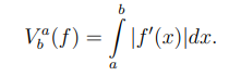
We interpret the total variation as a measure of the overall amount bet in a strategy. While it does not explicitly give the betting amount, it provides a metric for comparing stack functions. Some nice properties of total variation are Vba(f) = Vba(−f) and Vba(f) = Vba(f + c) for any function f and any constant c ϵ R. We use V(f) to denote the total variation of f on the domain of f.
Theorem 14
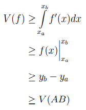
Let A = (xa, ya), B = (xb, yb) ϵ R2 with xa < xb. Let AB be the line segment connecting A to B. Let f be a differentiable function defined on [xa, xb] with f(xa) = ya and f(xb) = yb. Then
V(f) ≥ V(AB).
Proof: Case 1: ya ≤ yb. We first calculate V(AB). Since |AB'| = yb−ya / xb−xa then V(AB) = yb − ya. We now bound V(f)
Case 2: ya > yb. We reflect AB and f on the y = ya line. The reflection of f is fr(x) = 2ya − f(x), and the reflection of AB is ABr(x) = 2ya − AB(x). Similarly, |(ABr)'| = ya−yb / xb−xa, which implies that V(ABr) = ya − yb.

By properties of total variation, V(AB) = V(ABr) and V(f) = V(fr), which implies that V(AB) ≤ V(f).
Corollary 15
The stack function characterized by the line segment yoA minimizes total variation of all stack function exactly meeting the survival constraints.
Connection to Risk
Given a stack function P, increasing the aggressiveness of P increases the risk of P since the value bet is greater. The C1 norm contains the aggressiveness and the magnitude of the stack function. The greater the magnitude of a stack function, the more chips are bet and won or bet and lost to get to that critical point, which implies that a stack function P with greater C1 norm incurs greater risk. Similarly, if P has greater total variation, P acquires greater risk as more chips were bet. Since the stack function corresponding to the line segment y0A minimizes aggressiveness, the C1 norm, and total variation, we have the following conjecture:
Conjecture 16
The strategy corresponding to the stack function characterized by the line segment y0A minimizes risk.
CONCLUSION
We started this paper with concrete and practical results. However, these results not ideal the Zero Risk strategy minimizes risk, but it is not a feasible long term strategy. The linear programs provide a criterion for conservatively play, that is too survive longer in a tournament but not necessarily end with more chips. The linear programs do not completely minimize risk, and do not provide any insight on how to win. Since the concrete results were not ideal, we analyzed betting patterns in a more abstract setting by approximating the expected outcomes of strategies with continuous stack functions. While this analysis is not as concrete and not fully concluded, it is promising. Since strategies are finite sequences and there are only finitely many decisions a player can make, it is theoretically possible to iterate through all possible strategies and find the expected outcome of each strategy. If our conjecture is correct, then the strategy which best fits the line segment y0A would be the optimal minimal risk strategy.
ACKNOWLEDGMENTS
We would like to thank Carnegie Mellon University and the Summer Undergraduate Applied Mathematics Institute (SUAMI) program for hosting and funding our research. In particular, we would also like to thank Dr. Winger.
REFERENCES
Jensen, A. (2011). Lecture notes on difference equations. Available: http://people.math.aau.dk/ matarne/11-imat/notes2011a.pdf.
MAT 772, F. .-. L. . N., Fall Semester. (2011). The gnats and gnus document preparation system. http://www.math.usm.edu/lambers/mat772/fall10/lecture5.pdfl.
Mayers, D., & Suli, E. (2003). An introduction to numerical analysis. Cambridge University Press.
Tao, T. (2008). Function spaces. https://terrytao.files.wordpress.com/2008/03/function_spaces1.pdf.