

Author: Nirmish Singla, Ajay K. Singla, MD, and Joon S. Lee, PhD.
Institution: University of Michigan, Ann Arbor
Date: May 2008
ABSTRACT
Urinary tract obstruction is a common clinical problem involving the narrowing of the ureters or urethra. Current diagnostic methods are invasive and costly, and urologists are constantly seeking new, inexpensive, non-invasive measures to diagnose obstruction. The present study investigates diagnostic applications of computational fluid dynamics (CFD) to urinary tract obstruction for the first time. Various hypothetical models were initially created in Gambit 2.1.6, in which the physics of flow was evaluated based on varying geometries and conditions. These models presented short segments of the tract and possible effects of obstruction. Flow analysis was conducted in Fluent 6.1.22 by comparing contours of velocity, static pressure, dynamic pressure, total pressure, and wall shear stress to results predicted by flow theory. Realistic models of both healthy and obstructed urethras and ureters were then similarly created and simulated. CFD equations accurately predicted the expected flow characteristics through both hypothetical and realistic models. Comparison of the calculated urethral outlet velocity in the models, between 6.91 and 16.9 m/s at the urethral orifice, to human uroflowmetry data shows that the simulated conditions fall within the range of realistic human flow. The accuracy of the models suggests future clinical potential of using CFD with current techniques in human tract analysis, secondary flow effects, disease prevention, and non-invasive diagnosis.
INTRODUCTION
Urinary tract obstruction is a common problem causing urinary stasis as a result of urethral or ureteral constriction anywhere along the urinary tract. Frequent causes of obstruction include benign prostatic hyperplasia (BPH), prostate cancer, stones, urethral strictures, bacterial infections, and surgical trauma (Resnick and Sutherland 2004). In females, although less common, obstruction may arise from pregnancy complications, stones, or pelvic malignancies; urinary obstruction in children is often a direct result of congenital anomalies (Resnick and Sutherland 2004).
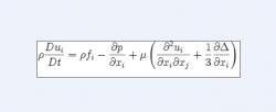
Equation 1 1518
Currently, diagnosis of obstruction can be performed by lab studies including urodynamic studies, imaging studies, or surgical procedures. Imaging studies, such as ultrasonography, computed tomography (CT) scans, and magnetic resonance imaging (MRI), are costly and time consuming (Resnick and Sutherland 2004), and the available results are limited to resolutions on the order of 1 mm due to issues of hardware, signal-to-noise ratio and acquisition time (Kim et al. 1997; Peled and Yeshurun 2001; Elad and Hel-Or 2001). Urodynamic studies and endoscopic procedures, such as cystoscopy, are invasive and may cause further complications (Resnick and Sutherland 2004). A numerical approach utilizing computational fluid dynamics (CFD) may eliminate such inconveniences.
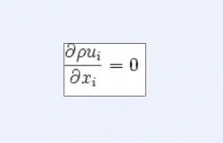
Equation 2
Much research in the field of mechanical engineering is concerned with flow through constricted tubes and its application to various organ systems. CFD modeling has been applied to the circulatory system in numerous ways involving flow effects of aneurysms, blood flow through stenoses (Siouffi et al. 1998; Blackburn and Sherwin 2005; Jung et al. 2004; Jou and Berger 2000), analysis of heart valves (Lim et al. 1980), and mechanics of arterial diseases (RuDusky 2003). CFD has also been applied to the respiratory system with regard to flow simulation and analysis (Luo et al. 2004). Fluid mechanics within the gastrointestinal tract have even been evaluated (Ooi et al. 2004). Such studies commonly involve the use of CFD software packages such as FLUENT, POLYFLOW, or FIDAP to perform model simulations and numerical analysis, along with compatible meshing software such as GAMBIT, TGRID, or G/Turbo to create the models themselves.

Equation 3
The present study investigates a novel technique of urinary tract simulation in both healthy and symptomatic patients using CFD and quantitatively evaluates the diagnostic potential of computerized models. In particular, Fluent 6.1.22 was used to simulate the flow mechanics inside the urinary tract, with emphasis on the effects of urinary tract obstruction, and flow was evaluated numerically by varying geometries and fluid properties. Applications of the models may include accurately predicting velocity and wall shear stress within the tract; extending the numerical simulation to include the secondary flow effects; determining whether flow analysis within the tract can help predict disease before it occurs; and creating a virtual diagnostic tool that applies CFD to the urinary tract for the first time.

Equation 4
METHODS
All models were created in Gambit 2.1.6 and simulated in Fluent 6.1.22. Contour plots and vectors of velocity, static pressure, dynamic pressure, total pressure, and wall shear stress were evaluated for each model, as such factors play a crucial role in clinical diagnosis. Path lines colored by particle identification and by velocity were also analyzed.

Equation 5
In Fluent, urine properties were assumed to be those of liquid water, as previously assumed (Cummings et al. 2004). The following properties of liquid water, obtained from the Fluent solver, were used for Reynolds number calculations: density=998.2 kg/m3 and viscosity=0.001003 kg/(m*s). In the laminar model, second-order pressure and upwind momentum were used to minimize truncation and discretization errors. For turbulence modeling, the standard k- solver was used, and second-order upwind was used for both k and . Two major types of models were created: hypothetical and realistic.

Equation 6
Hypothetical Models
The hypothetical models presented short segments of the urinary tract and potential geometric representations of obstruction. In these models, more attention was paid towards investigating the physics of flow and its dynamicity, based on variable geometries and boundary conditions. For all simulated models, Reynolds number was varied and simulated in the appropriate solver. Reynolds values of 700 and 5,000 were compared; inlet velocities were calculated to be 0.1406732 and 1.0048087 m/s, respectively, using Equation 6. Each model was further enhanced to more precisely apply to the human urinary tract.

Equation 7
2D Cases
Initially, a 2D cross-sectional model was created (Figure 1) as a control. A Venturi with diameter of 5 mm was used, and constriction was moderate (1.5 mm deep, 3 mm wide). The inlet edge designated the velocity inlet and the outlet edge the pressure outlet; such would yield fluid flow in the positive x direction with a specified velocity inlet. This model was then simulated in Fluent.
Equation 8
The effect of varying the horizontal distance between the two constrictions from Figure 1 was initially observed by considering several cases of varying distance; for example, Figure 2 presents the case in which the distance is 6 mm. The effect of constriction severity was also observed, with mildly and severely constricted models; both constriction depth and width were considered. Finally, the effect of multiple constrictions and varying distances between them was studied, as shown in Figure 3.
3D Cases
To construct the 3D cases, each of the 2D models was rotated 360 degrees about its horizontal axis of symmetry (y=2.5); Figure 4, for example, shows a 360-degree rotation of Figure 1. The 2D cases of variable constriction severity, constriction multiplicity, and distance between constrictions were rotated in a likewise fashion and simulated.
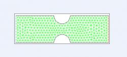
Figure 1. Two-dimensional cross section of control grid with symmetric constriction. Venturi diameter was 5 mm and constriction diameter was 1.5 mm deep and 3 mm wide (moderate). Green lines represent triangular mesh, blue line designates velocity inlet, and red line designates pressure outlet. Model was created in Gambit for subsequent simulation in Fluent.

Figure 2. Two-dimensional cross section of grid with variable distance between constrictions, relative to control case. Specifically shown, a distance of 6 mm spans between two moderate constrictions (1.5 mm deep, 3 mm wide). Green lines represent triangular mesh, blue line designates velocity inlet, and red line designates pressure outlet. Model was created in Gambit for subsequent simulation in Fluent.
Grid Independence Test
To ensure consistency in the models, it is important that a grid independence test be performed for both 2D and 3D cases, as a finer grid yields greater accuracy. Such a test decreases the mesh spacing to a point such that further decreasing the interval would have a negligible effect on the outcome of a simulation while minimizing time and memory consumption. In the 2D case, a triangular mesh was used with a symmetric Venturi, while in the 3D case, a tetrahedral mesh was used. Mesh spacings of 1, 0.5, 0.25, and 0.125 were assayed with regard to velocity in the turbulence model, and an interval spacing of 0.5 was ultimately selected for all 2D and 3D cases.
Realistic Models
In the realistic models, complete ureters and urethras were modeled. Both healthy and obstructed models were created and compared to experimental data to assess accuracy. In Fluent, an inlet velocity of 0.284 m/s (Re=2,826.409 for liquid water using Equation 6) was used for the ureter, and 1.166 m/s (Re=9,556.400) was used for the urethra, based on realistic urine velocity data obtained in humans (Hashimoto 1992). The standard k- model was used for all realistic simulations.
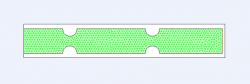
Figure 3. Two-dimensional cross section of grid with multiple constrictions and variable distances between them. The effects of both constriction severity (depth, width) and distance were assessed. Specifically shown, two constrictions with a medium spanning distance and moderate constriction (1.5 mm deep, 3 mm wide). Green lines represent triangular mesh, blue line designates velocity inlet, and red line designates pressure outlet. Model was created in Gambit for subsequent simulation in Fluent
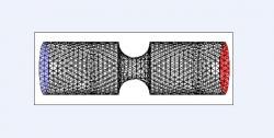
Figure 4. Three-dimensional control grid with symmetric constriction. Venturi diameter was 5 mm and constriction diameter was 1.5 mm deep and 3 mm wide (moderate). Model was created in Gambit by rotating respective two-dimensional cross sectional grid 360 degrees about the horizontal line of symmetry. Black lines represent tetrahedral mesh, blue face designates velocity inlet, and red face designates pressure outlet. Model was subsequently simulated in Fluent.
Ureter
A ureteral model was created from scaling an anatomical diagram (available at http://www.uco.org.au/images/urology.swf, Urological Cancer Organisation) of the urinary system; the scale ratio was measured to be 10:1. Additional anatomical information regarding specific lengths, bends and diametric narrowings (Standring 2005) were used to establish Cartesian coordinates to be plotted in Gambit (Table 1).
Coordinates were labeled A1-G1 and A2-G2, as displayed in Table 1. Edge A1A2 was the ureteropelvic junction (UPJ) and velocity inlet, and edge G1G2 was the ureterovesical junction (UVJ) and pressure outlet. The abdominal ureter length spanned from A1A2 to C1C2, and the pelvic ureter from C1C2 to G1G2. The coordinates were connected via non-uniform Rational B-Splines (NURBS). All edges other than A1A2 and G1G2 were walls. A triangular mesh of 0.5 spacing was used to create the healthy 2D ureteral model (Figure 5).

Figure 5. Two-dimensional cross sectional healthy model of the ureter, created via a 10:1 anatomical scaling in Gambit. Cartesian coordinates used are presented in Table 1. Coordinates were labeled A1-G1 and A2-G2. Green lines represent triangular mesh (0.5 spacing, determined by grid independence test), blue line designates velocity inlet (ureteropelvic junction, edge A1A2), and red line designates pressure outlet (ureterovesical junction, edge G1G2). Abdominal and pelvic segments of ureter connect at C1 and C2. Non-uniform Rational B-Splines were used to connect ureter walls, A1G1 and A2G2. Model was subsequently simulated in Fluent.
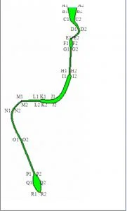
Figure 6. Two-dimensional cross sectional healthy model of male urethra, created via a 20:17 anatomical scaling in Gambit. Cartesian coordinates used are presented in Table 2. Coordinates were labeled A1-R1 and A2-R2. Green lines represent triangular mesh (0.5 spacing, determined by grid independence test), blue line designates velocity inlet (bladder neck, edge A1A2), and red line designates pressure outlet (urethral orifice, edge R1R2). Prostatic urethra conjoins membranous urethra between points G and H, and membranous urethra conjoins spongy (penile) urethra at point H. Navicular fossa is encompassed by segment PR. Non-uniform Rational B-Splines were used to connect urethra walls, A1R1 and A2R2. Model was subsequently simulated in Fluent.
3D
The 2D model could not be revolved 360 degrees about its center, as Gambit prohibits revolution of faces about a twisted or scrunched edge. Instead, skin surfaces in the z-plane were created and combined. The volume could not be meshed using a tetrahedral mesh, so a hexahedral mesh with a Cooper meshing scheme and 0.5 spacing was used. Although the mesh was successfully exported to Fluent, the grid check failed and immediate divergence was detected; the model could not be simulated in Fluent.
Obstructed Models
Three areas of the ureter are most susceptible to obstruction: the UPJ, UVJ, and the abdomino-pelvic ureteral junction (Resnick and Sutherland 2004). For UPJ obstruction, segment A1A2 was reduced to 1 mm; all other factors were held constant. For obstruction at the abdomino-pelvic junction, C1C2 was reduced to 1 mm. For UVJ obstruction, G1G2 was reduced to 0.5 mm.

Figure 7. Flow characteristics in laminar solver (Fluent) for two-dimensional control Venturi. Reynolds number was 700 based on inlet velocity, and constriction was of moderate severity (1.5 mm deep, 3 mm wide). The effect of the constriction on velocity, static pressure, dynamic pressure, and total pressure are shown by respective contour plots. Blue contours represent minimal (zero) values, while red contours represent maximal values. Velocity and dynamic pressure display maximal values at site of constriction, whereas static pressure is at a minimum. Note that, despite the laminar flow profile, contours appear to drift upwards, possibly an effect of flow that has not developed fully.

Figure 8. Flow characteristics in turbulent standard k-epsilon solver (Fluent) for two-dimensional control Venturi. Reynolds number was 5,000 based on inlet velocity, and constriction was of moderate severity (1.5 mm deep, 3 mm wide). The effect of the constriction on velocity, static pressure, dynamic pressure, and total pressure are shown by respective contour plots, and are shown for comparison to fluid dynamics of the same model in the laminar solver (Re=700). Blue contours represent minimal (zero) values, while red contours represent maximal values. As in the laminar solver, velocity and dynamic pressure display maximal values at site of constriction whereas static pressure is at a minimum. However, the non-symmetric distribution of contours is a result of the turbulent nature of the flow. Underdeveloped flow may also contribute to the observed distribution.
Urethra
A urethral model was created from scaling a male urethra in a similar fashion as used for the ureter (available at http://ect.downstate.edu/courseware/haonline/figs/l44/440408.htm, SUNY Downstate Medical Center); the scaled ratio was measured to be 20:17. As males are more susceptible to urethral obstruction than females, only models of the male urethra were created. Additional anatomical information regarding specific lengths, bends and diametric narrowing (Standring 2005) was used to establish Cartesian coordinates to be plotted in Gambit (Table 2). Each coordinate in the table was multiplied by 20/17 before plotting to account for the scale ratio.
Coordinates were labeled A1-R1 and A2-R2. Segment A1A2 was the bladder neck and velocity inlet. The prostatic urethra spanned from A1A2 to the midpoint of segments G1G2 and H1H2. The membranous urethra followed the prostatic for 15 mm, until segment H1H2. The spongy or penile urethra spanned from H1H2 to P1P2 (bulbar from H1H2 to L1L2 and non-bulbar from L1L2 to P1P2), and J1J2 represented the first angle or bend. P1P2 to R1R2 represented the navicular fossa, and the urethral orifice (R1R2) was a pressure outlet. The coordinates were connected via NURBS, and edges other than A1A2 and R1R2 were walls. A triangular mesh with 0.5 spacing was used to create the 2D healthy model (Figure 6).

Figure 9. Velocity contours of two-dimensional cross section of healthy ureter, simulated in turbulent standard k-epsilon solver (Fluent). Contours are shown for the ureter as a whole (a), and for magnified region at the ureteropelvic junction (UPJ, inlet) (b) and ureterovesical junction (UVJ, outlet) (c). Blue contours represent minimal (zero) values, while red contours represent maximal values of velocity. Trend indicates a steady increase in urine velocity throughout the ureter from the UPJ to the UVJ, due to natural narrowing of the diameter.

Figure 10. Velocity contours of two-dimensional cross sections of obstructed cases of the ureter, simulated in turbulent standard k-epsilon solver (Fluent). As shown, contours are magnified at the outlets (ureterovesical junction) for the cases of UPJ constriction (a), constriction at the abdomino-pelvic junction (b), and UVJ constriction (c). Blue contours represent minimal (zero) values, while red contours represent maximal values of velocity. Compared to the healthy ureter, constricted cases displayed decreased ureteral outflow, notable especially in the cases of UPJ and UVJ constriction.
3D
Gambit prohibited a 360-degree revolution of the 2D model. An attempt was made to create a 3D model in a similar fashion as in the ureteral model. However, creation of a skin surface in the z-plane could not be completed. An attempt to create multiple volumes along the tract by revolving individual segments by 360 degrees and subsequently merging them also failed. A 3D model was unable to be created in Gambit using the employed methods.
Obstructed Models
Three areas of the urethra are most susceptible to obstruction: the bladder neck, prostatic urethra and first angle (bulbar spongy urethra) (Resnick and Sutherland 2004). 2D cross-sectional models for each obstructed case were created and simulated.
For the obstructed bladder neck case, the inlet diameter was reduced to 0.5 mm. All other factors were held constant. Benign prostatic hyperplasia (BPH), prostate cancer, or other diseases of the prostate gland may cause constriction along the prostatic urethra. For this model, the diameter of the prostatic urethra was reduced to 0.5 mm. Obstruction at the first angle occurs in the bulbar portion of the spongy urethra. In the model of first angle obstruction, the bulbar penile urethra diameter was reduced to 1 mm. All models were simulated.

Figure 11. Velocity contours and vectors of two-dimensional cross section of healthy urethra, simulated in turbulent standard k-epsilon solver (Fluent). Contours are shown for the urethra as a whole (a) and magnified at the bladder neck (b). Vectors are shown for magnified region at the navicular fossa and urethral orifice (c) to display circulatory nature of flow. Blue contours represent minimal (zero) values, while red contours represent maximal values of velocity. Trend displays increased velocities in narrower regions of the urethra, as expected, with outlet velocity slightly greater than at the inlet.
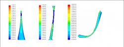
Figure 12. Velocity contours of two-dimensional cross section of obstructed cases of the urethra, simulated in turbulent standard k-epsilon solver (Fluent). As shown, contours are magnified at respective sites of constriction. Specifically displayed are the cases for bladder neck obstruction (a), benign prostatic hyperplasia (BPH) (b), and bulbar spongy urethral (first-angle) constriction (c). Blue contours represent minimal (zero) values, while red contours represent maximal values of velocity. Trends illustrate that velocity continues to increase as diameter narrows; however, depending on the severity of the constriction, as the diameter continues to narrow, the effects of wall shear stress generated on each side of the tract converge, thereby causing velocity to drop instantaneously to zero (complete obstruction).
RESULTS
Hypothetical Models
In the hypothetical models, fluid dynamics were evaluated with regard to velocity, static pressure, dynamic pressure, and total pressure. Path lines and contour plots indicated a decreased output of urine in response to greater magnitudes of constriction. Figure 7 displays the flow characteristics in the 2D cross-sectional control Venturi model with moderate constriction severity utilizing a laminar solver (Reynolds value of 700). By comparison, Figure 8 displays flow characteristics in the control model utilizing a turbulent solver (Reynolds value of 5,000). Numerical values of velocity and pressure derived from these models, with particular focus on the flow at the inlet, constricted, and outlet regions, are tabulated in Table 3. Values presented in Table 3 are representative approximations based on contour plot scales.
The data indicates similar trends between the laminar and turbulent solvers. In particular, greater velocities and dynamic pressures were noted at constricted regions relative to those at the inlet along with corresponding negative static pressures, as observed in Table 3. For example, in the laminar solver, an inlet velocity of 0.141 m/s corresponds to a constriction velocity of 0.356 m/s, approximately a 2.5-fold difference. Likewise, a constriction velocity of 2.40 m/s in the turbulent solver corresponds to a 2.4-fold difference over the inlet velocity of 1.00 m/s, illustrating similarity between the trends in the two solvers.

Table 1. Cartesian coordinates used for two-dimensional cross section of healthy ureteral grid, determined via a 10:1 anatomical scaling in Gambit in conjunction with specific anatomical parameters. Coordinates were labeled A1-G1 and A2-G2 and connected via non-uniform Rational B-Splines, as displayed in Figure 5. Both the abdominal and pelvic segments of the ureter are included.

Table 2. Cartesian coordinates used for two-dimensional cross section of healthy urethral grid, determined via a 20:17 anatomical scaling in Gambit in conjunction with specific anatomical parameters. Note that each coordinate displayed in the table was multiplied by a factor of 20/17 prior to plotting in Gambit. Coordinates were labeled A1-R1 and A2-R2 and connected via non-uniform Rational B-Splines, as displayed in Figure 6. Anatomical segments included in the model are the prostatic urethra, membranous urethra, spongy (penile) urethra (both bulbar and non-bulbar), first angle (bend), and navicular fossa.
Table 4 displays the effect of constriction severity on the control model for mild, moderate, and severe cases of obstruction. The data illustrates a direct correlation between velocity, pressure magnitudes, and constriction severity.
The effect of varying distances between constrictions in a doubly-constricted case (as in Figure 3) displayed no significant effect on flow characteristics. Contours of velocity and pressure at the corresponding regions of constriction were shown to be similar in the cases with a smaller gap between constrictions and those with larger gaps. Furthermore, outlet flow conditions were similar to those observed in the control case.
Realistic Models
Ureter
In the realistic models, more emphasis was placed on contours of velocity, from which pressure contours could be deduced. Figure 9 displays the velocity contours observed in the healthy ureteral model, magnified at the inlet and outlet. Velocity increased steadily throughout the tract from the UPJ to the UVJ. Figure 10 displays the velocity contours at the UVJ for the cases of UPJ, abdomino-pelvic ureteral, and UVJ obstruction. Inlet and outlet velocities are tabulated for each case in Table 5. Selected inlet values of 0.284 m/s converged in all cases.
The data demonstrates that all diseased states decreased ureteral outflow. In particular, whereas the case of abdomino-pelvic ureteral constriction only slightly decreased outlet velocity, UPJ and UVJ constriction had more profound effects.

Table 3. Numeric flow data for two-dimensional cross section of control Venturi comparing the laminar (Re=700) and turbulent standard k-epsilon (Re=5,000) cases (Fluent). Shown are the approximate measured contour values for velocity (in m/s), static pressure, dynamic pressure, and total pressure (in Pa) at the inlet, outlet, and site of constriction, as depicted in Figures 7 and 8. Note that in some cases, a range of values, rather than a single value, more accurately depicted the transverse variability in certain variables. Significantly higher magnitudes of velocity and pressure were measured in the turbulent case as compared to the laminar case because inlet velocities needed to be greater to accommodate larger Reynolds values. From the relative velocities at the site of constriction, an inverse relationship between velocity and diameter illustrates the validity of conservation of mass.
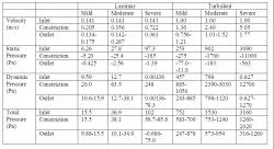
Table 4. The quantitative effect of variable constriction severity on flow characteristics for the two-dimensional symmetric Venturi cross-section. Numeric data for velocity (in m/s), static pressure, dynamic pressure, and total pressure (in Pa) at the inlet, outlet, and site of constriction are shown for both the laminar (Re=700) and turbulent standard k-epsilon (Re=5,000) cases (Fluent). Compared to the control case of moderate constriction severity (1.5 mm deep, 3 mm wide), mild and severe cases were analyzed. Note that in some cases, a range of values, rather than a single value, more accurately depicted the transverse variability in certain variables. Higher inlet velocities were specified in the turbulent solver to accommodate larger Reynolds values. The trend indicates an overall direct correlation between velocity, the magnitudes of pressure, and constriction severity, as expected.
Urethra
Contours and vectors of velocity are shown for the healthy urethral model (Figure 11) with magnifications at the bladder neck (inlet) and navicular fossa (outlet). An inlet velocity of 5.0 m/s was specified in the healthy model for convergence of the solver. Corresponding velocity contours in each of the obstructed cases at the sites of constriction,bladder neck constriction, BPH, and bulbar spongy urethral constriction,are displayed in Figure 12. Inlet and outlet velocities are tabulated in Table 6 for each case.
Table 6 indicates relatively higher outlet flow velocities in comparison to those at the inlets in all cases except for bladder neck constriction. Additionally, only the case of bulbar spongy urethral obstruction could converge at the anticipated 1.166 m/s inlet value. All other cases required a higher inlet velocity specification in Fluent.
DISCUSSION

Table 5. Measured inlet and outlet velocities in two-dimensional cross sectional models of both healthy and obstructed cases of the ureter, simulated in turbulent standard k-epsilon solver (Fluent). Specific locations of obstruction were at the ureteropelvic junction, abdomino-pelvic junction, and ureterovesical junction. Inlet velocity of 0.284 m/s converged in all cases. Data indicates decreased ureteral outflow as a result of disease, especially notable in the cases of UPJ and UVJ constriction. *Note that in the case of UVJ constriction, due to the severity of constriction, the outlet velocity was measured to be zero because of the converging effects of wall shear stress generated from the two sides of the tract. Prior to complete flow obstruction, the flow displayed a velocity range between ~2.98 m/s and 4.26 m/s.
A recent study (Martinez-Borges 2006) proposed turbulent urinary flow as a causal factor of BPH, suggesting the necessity to conduct investigations of urethral fluid dynamics. Previous studies have developed both quantitative and computerized models to assess the flow of urine in the lower urinary tract. For example, Valentini et al. developed a computerized mathematical micturition model capable of analyzing physiological changes during voiding (2000) and applied their model to benign prostatic enlargement using pressure-flow analysis (2003). However, the Valentini-Besson-Nelson model focuses more on physiological uroflow curve interpretation. Ohnishi et al. evaluated theoretical possibilities of lower urinary tract simulation using a hydrodynamic model (1991); similar quantitative studies regarding urodynamic models and pressure-flow analysis have been suggested as well (Chamorro et al. 1998; Witjes et al. 2002; van Mastrigt and Kranse 1992; Pel and van Mastrigt 2007), with slightly different objectives.
Hypothetical Models

Table 6. Measured inlet and outlet velocities in two-dimensional cross sectional models of both healthy and obstructed cases of the urethra, simulated in turbulent standard k-epsilon solver (Fluent). Specified locations of obstruction were at the bladder neck, prostatic urethra (benign prostatic hyperplasia, BPH), and spongy urethra. An inlet value of 5.0 m/s enabled convergence in the healthy model. An inlet velocity of 1.166 m/s converged only in the case of bulbar spongy urethral constriction. With the exception of the case of bladder neck constriction, the data indicates relatively higher outlet flow velocities (as compared in magnitude to the specified inlet values).
Flow proved consistent with CFD equations and basic fluid flow theory. The Navier-Stokes conservation of mass equation, Equation 2, explains the inverse relationship between velocity and area, and hence why the velocity at constricted points was relatively greater than at the inlet. The Navier-Stokes conservation of momentum equation, Equation 1, relates velocity and pressure, and the Bernoulli equation, a simplification of the Navier-Stokes equations, further explains the static-dynamic pressure relationships. The Newtonian quality of urine explains the direct relationship between velocity and wall shear stress.
Figures 7 and 8 indicate that the flow was not symmetric despite symmetric geometry. This may be a result of body force. Reversed flow was present in some models. The concept of fully developed flow was considered for eliminating such flow, and Equations 7 and 8 were used to determine the necessary entrance length for the flow to fully develop (210 mm inlet for Re=700 and 90.974 mm inlet for Re=5,000). The models were modified, and reversed flow was eliminated.
The 3D cases were evaluated in a similar fashion as the 2D cases. Although slight differences were noticed between 2D and 3D results, such differences were expected due to differences in the equations used by the two Fluent solvers. 3D cases had also taken secondary flows into account. Further, convergence in the laminar solver was restricted in most models for both Reynolds values, possibly due to geometric complexity. All 3D models were simulated in the turbulence solver, but results proved quite similar to those of the 2D models.
Realistic Models
Ureter
CFD equations accurately predicted the flow through the healthy and obstructed ureteral models with regard to diametric changes, as illustrated by velocity contours in Figures 9 (a-c) and 10 (a-c). Greater relative outlet and constriction velocities were observed and expected, due to the natural diametric narrowing of the tract. Additionally, similarities between 2D and 3D hypothetical model results indicate that the 2D ureteral models can accurately represent 3D cases of the ureter that could not be simulated.
Interestingly, in UVJ obstruction (Figure 10 (c)), the velocity increased before the outlet until a certain point, after which it became zero. The data indicates that the effect of wall shear stress, initiated by the Newtonian property of urine, increased until a point at which the effect of the two walls converged due to the severity of the constriction. Such suggests that, under the given boundary and operating conditions, urine would be unable to flow beyond the point of obstruction unless ureteral pressure is increased.
Urethra
In both the healthy and obstructed urethral models, flow was also predictable, based on velocity-area relationships (greater velocity at the urethral orifice than at the bladder neck) and decreased output from constriction, as seen in Figures 11 (a-c) and 12 (a-c). In the cases of bladder neck obstruction and BPH, stagnant flow was observed, similar to the case of UVJ obstruction. Again, this was caused by constriction severity and wall shear stress and can be eliminated by increasing detrusor pressure. In the model of first-angle constriction, however, since the constriction was not as severe, there was no stagnant flow under the simulated conditions.
Interesting results were obtained from varying inlet velocities in all models. In the healthy model, a floating point error was detected at an inlet velocity of 1.166 m/s, and the solution did not converge. Inlet velocity was varied and assayed at increasing integer quantities until convergence, which occurred at 5 m/s (as in Figure 11). An inlet velocity of 4.5 m/s (Re=36,881.473) diverged, but an inlet of 4.51 m/s (Re=36,963.432) converged, indicating a potential relationship between Reynolds number, geometry, and convergence. Detrusor pressure possibly accounts for the higher inlet velocity, as such would enable urine flow from inlet to outlet.
However, the solution also converged at inlet values less than 0.1 m/s. It is possible for involuntary flow (leaks) to occur in incontinent patients, in which the flow velocity is typically much less than in healthy patients, yet relative fluid dynamics remain consistent. Such is a possibility for the lower inlet values. Varying the inlet velocity only affected the circulatory flow within the navicular fossa, while flow throughout the rest of the urethra, including the orifice, remained consistent. A Re-Normalization Group (RNG) k- solver would be better for circulatory flow analysis than the standard k- model, as the RNG equations would more accurately model swirling flow.
In the bladder neck obstruction and BPH models, even greater velocity inlets were required for convergence, as expected. Interestingly, for the first-angle case, however, the flow converged at an inlet of 1.166 m/s. A possible explanation is that in the healthy model, the bulbar urethral diameter was so great that a greater Reynolds number was necessary for convergence, but in the first-angle constriction case, since the diameter of the bulbar urethra was reduced, the Reynolds number calculation was affected, yielding the possibility of convergence at 1.166 m/s. Supposedly, if a more severe case of first-angle constriction were used, then an inlet of 1.166 m/s would not converge. Theoretical analysis was assessed using CFD equations and flow theory; however, further accuracy in a clinical setting can be evaluated by comparing Fluent results to experimental uroflowmetry data.
Comparison to Experimental Data and Clinical Applications
Normal uroflow volume rates in men between 4 and 80 years of age range from 9 to 21 cm3/sec, depending on age (Gilbert 2004). To calculate the outlet velocity in cm/sec, uroflow values were divided by the cross sectional area of the outlet (in cm2). A urethral orifice radius of 0.088235 cm was used in the healthy urethral model, yielding an orifice area of 0.024446 cm2. Realistic outlet velocities hence range from 368.158 cm/sec (3.68 m/s) to 859.036 cm/sec (8.59 m/s) with the given parameters. Figure 11 (c) indicates that an inlet velocity of 5 m/s yielded outlet velocities between 6.91 and 16.9 m/s, which are slightly higher than predicted. This suggests that increasing the diameter of the urethral models and decreasing the inlet velocity would yield more realistic outlet values. Nonetheless, accurate modeling of the urinary tract with the given procedures is restricted by variation in urinary tract parameters and in the urethral lumen diameter (wall compliance).
Clinically, the CFD models may extend the current diagnostic potential of uroflowmetry tests by incorporating such factors as static and dynamic pressure as well as velocity output. By analyzing the differences in outlet flow values for each case of obstruction, the models can be used in conjunction with current imaging techniques to potentially pinpoint the exact location and type of urinary obstruction in patients. Additionally, each model can be varied to model patient-specific urinary tract parameters for more precision in clinical applications.
Challenges and Limitations for Future Consideration
Indeed, several points of concern exist for future improvements. Additional experimental data must be obtained for greater accuracy. For example, determining the density and viscosity of urine would alter Reynolds number calculations and yield more realistic results. Further minimization of truncation and discretization errors as well as reversed flow would even further improve accuracy. Convergence difficulties in the laminar and turbulent solvers and difficulties in the grid independence tests for very fine meshes still require further investigation. The chosen turbulent solver (standard k-ε) may be varied for additional accuracy; for example, use of the RNG k- solver would provide greater precision in the analysis of swirling flows.
Creation of the models was based on a Cartesian approach in Gambit, which limits realistic modeling, especially in the 3D cases. Urinary tract walls were also rigid in Fluent, whereas the human urinary tract displays wall compliance. Programs other than Gambit and Fluent, such as Amira and ADINA, respectively, are currently being investigated to simulate MRI's and CT scans of the tract using fluid-structure interaction (FSI). Such programs may present a drawback, however, as MRI's and CT scans do not typically cover the complete urinary tract and the cropping and exportation processes would require numerous hours. Nonetheless such programs would provide for more patient-specific variation in urinary tract parameters.
The present study analyzed the fluid dynamics of urine inside the urinary tract. The flow was evaluated through constricted tubes, and attention was paid to the effects of such constriction and to variable geometries and fluid properties. For the first time, CFD was applied to the urinary tract as a whole to create a non-invasive diagnostic tool for urinary tract obstruction in both the ureter and urethra. The models have implications for clinical applications of urinary tract analysis, secondary flow effects, diagnosis, and possible disease prevention by early detection.
REFERENCES
Blackburn, HM and SJ Sherwin (2005) Three-dimensional instabilities and transition of steady and pulsatile axisymmetric stenotic flows. J Fluid Mechanics 533(1), 297-327.
Chamorro, MV et al. (1998) Urodynamic models in the analysis of pressure-flow studies in the adult male. Arch Esp Urol 51(10), 1011-1020.
Cummings, LJ et al. (2004) The effect of ureteric stents on urine flow: reflux. J Math Biol 49, 56-82.
Elad, M and Y Hel-Or (2001) A Fast Super-Resolution Reconstruction Algorithm for Pure Translational Motion and Common Space Invariant Blur. IEEE Trans Image Process 10(8), 1187-1193.
Gilbert, SM (2004) Uroflometry. MedlinePlus Medical Encyclopedia. U.S. National Library of Medicine, National Institutes of Health, http://www.nlm.nih.gov/medlineplus/ency/article/003325.htm.
Hashimoto, T et al. (1992) Visualization of the intravesical urine stream. Hinyokika Kiyo 38(5), 531-534.
Jou, LD and SA Berger (2000) Flows in stenotic vessels. Ann Rev Fluid Mechanics 32, 347-382.
Jung, H et al. (2004) Asymmetric flows of non-Newtonian fluids in symmetric stenosed artery. Korea-Australia Rheology Journal 16(2), 101-108.
Kim, SG et al. (1997) Limitations of Temporal Resolution in Functional MRI. Magn Reson Med 37(4), 631-636.
Lim, K et al. (1980) Analysis of mitral and aortic valve vibrations and their role in the production of the first and second heart sounds. Phys Med Biol 25(4), 727-733.
Luo, XY et al. (2004) LES modelling of flow in a simple airway model. Medical Engineering and Physics 26(5), 403-413.
Martinez-Borges, AR (2006) Turbulent urinary flow in the urethra could be a causal factor for benign prostatic hyperplasia. Medical Hypotheses 67(4), 871-875.
Ohnishi, K et al. (1991) A study of the simulation model of the lower urinary tract for urodynamics--(the first report)--theoretical evaluation of hydrodynamic model. Hinyokika Kiyo 37(10), 1249-1253.
Ooi, RC et al. (2004) The flow of bile in the human cystic duct. J Biomechanics 37, 19131922.
Pel, JJM and R van Mastrigt (2007) Development of a CFD urethral model to study flow-generated vortices under different conditions of prostatic obstruction. Physiol Meas 28, 13-23.
Peled, S and H Yeshurun (2001) Superresolution in MRI: Application to Human White Matter Fiber Tract Visualization by Diffusion Tensor Imaging. Magn Reson Med 45, 29-35.
Resnick, M and S Sutherland (2004) Urinary Tract Obstruction. eMedicine Clinical Knowledge Base. WebMD, http://www.emedicine.com/med/topic2782.htm.
RuDusky, BM (2003) Mechanical factors in the production of atheromatous disease with a critique on antilipid therapy. Cardiovascular Engineering: An International Journal 3(1), 39-44.
Siouffi, M et al. (1998) Experimental analysis of unsteady flows through a stenosis. J Biomechanics 31, 11-9.
Standring S. 2005. Gray's Anatomy: The Anatomical Basis of Clinical Practice, 39th ed. New York: Churchill Livingstone. 1600 p.
Valentini, FA et al. (2000) A mathematical micturition model to restore simple flow recordings in healthy and symptomatic individuals and enhance uroflow interpretation. Neurourol Urodyn 19(2), 153-176.
Valentini, FA et al. (2003) Modelized analysis of pressure-flow studies of patients with lower urinary tract symptoms due to benign prostatic enlargement. Neurourol Urodyn 22(1), 45-53.
van Mastrigt, R and M Kranse (1992) Analysis of pressure-flow data in terms of computer-derived urethral resistance parameters. World J Urol 13(1), 40-46.
Witjes, WP et al. (2002) Computerised assessment of maximum urinary flow: an efficient, consistent, and valid approach. Eur Urol 41(2), 205-213.
Appendix: Governing Equations and Additional Formulas
Urine is a Newtonian fluid, one in which there is a simple, linear relationship between shear stress and the velocity gradient. Viscous, incompressible Newtonian fluids are governed by the Navier-Stokes equations (Equations 1, 2, and 3). In these equations, ρ is the density, ui (i = 1,2,3) are the three components of velocity, fi are body forces (such as gravity), p is the pressure, and μ is the constant viscosity of the fluid. Such equations were applicable since the viscosity and density of the working fluid were treated as a constant.
The standard k-epsilon (k-ε) model was used for assessing turbulent flow. This model is appropriate for fully-turbulent flows in which molecular viscosity is negligible. Two transport equations (Equations 4 and 5) are involved in this model, from which turbulence kinetic energy, k, and its dissipation rate, ε , can be obtained. In these equations, Gk is the generation of turbulence kinetic energy due to the mean velocity gradients; Gb is the generation of turbulence kinetic energy due to buoyancy; Ym represents the contribution of the fluctuating dilatation in compressible turbulence to ε; C1ε, C2ε, and C3ε are constants; σK and σε are the turbulent Prandtl numbers for k and ε, respectively; and SK and Sε are user-defined source terms. The solver was chosen as it is the most practical and basic solver for engineering and CFD applications and purposes.
The Reynolds number (Re), defined in Equation 6, is used to determine whether flow is laminar (usually Re < 2,000 for an internal flow), turbulent (usually Re > 4,000 for an internal flow), or transitional (2,000 less than or equal to Re which is less than or equal to 4,000). As Re is just an approximation, determination of turbulence varies with other factors, such as geometric complexity.
A flow must be fully-developed within a tube before a constricted area in order to ensure accuracy. The formulas for the inlet length of a tube for full flow development are based on Re (laminar or turbulent flow) and tube diameter, as shown in Equations 7 and 8.
ACKNOWLEDGEMENTS
Access to Fluent 6.1.22 and Gambit 2.1.6 provided by the CFD laboratory in the Department of Mechanical Engineering at Wayne State University is gratefully acknowledged. Appreciation is given to mentors Joon Sang Lee, PhD (Department of Mechanical Engineering, Wayne State University) and Ajay Kumar Singla, MD (Department of Urology, Wayne State University) for their technical assistance throughout the duration of the present work.