Cerebrospinal Fluid-Tissue Interactions in the Human Brain

Author:  Kirstin Tawse

Institution:  Laboratory for Product and Process Design, University of Illinois at Chicago
Date:  May 2008

ABSTRACT

The dynamic interaction between the solid brain, cerebrospinal fluid and blood flow within the cranial vault have previously been described only qualitatively. In this study, computational analysis using the finite element method and physiological parameters was used to describe cerebrospinal fluid-tissue interactions in a quantitative manner. By describing the soft tissue deformations and fluid flow under both normal and pathological conditions, we were able to quantify human intracranial dynamics with the hope of allowing prediction of pathophysiological conditions leading to hydrocephalus or other cerebral disease states.

MRI images of the cranial vault were converted to a discretized mapping of finite elements. Physical principles of fluid flow and solid mechanics in addition to known physiological parameters were then applied to these actual human geometries. The numerical solution for fluid motion and solid deformation over this discretized brain geometry was then obtained using a commercial solver. In a series of three case studies it was found that a large transmural pressure difference was not necessary in order to produce hydrocephalic like ventricular distension, thus validating previous work that claimed no large pressure difference between the ventricles and subarachnoid space existed in communicating hydrocephalus (Linninger et al. 2005). It was also shown that the application of pressure to the solid brain could induce a fluid flow within the porous brain, indicating that under such conditions a net shift in brain water content may occur. Finally, it was shown that the vasculature system could induce a net motion of the solid brain which in turn induced the pulsatile cerebrospinal fluid flow previously observed using MRI, thus validating the brain motion hypothesis (Greitz 2006). In all of the case studies it was found that cerebrospinal fluid-tissue interactions are a primary factor in the determination of intracranial dynamics.

It is recommended that future studies further investigate pathological-like cerebrospinal fluid (CSF) flow patterns and tissue deformations through the application of parameters consistent with possible cerebral disease confounders (e.g. decreased brain tissue compliance).

INTRODUCTION

Intracranial dynamics is defined as the interaction between solid brain tissue, cerebrospinal fluid (CSF) (colorless liquid within which the brain and spinal cord are submerged), and blood flow throughout the central nervous system. CSF has been found to flow between hollow cavities within the brain known as ventricles and fluid filled spaces surrounding the brain and spinal cord known as the subarachnoid space (SAS). It has also been observed that the flow of CSF occurs in a pulsatile manner in synchronization with the cardiac cycle. Production of CSF occurs predominantly at the choroid plexus located within the ventricles as well as to a lesser degree from arterial capillaries within the parenchyma of the brain (Rekate et al. 1985; Linninger et al. 2007). Expansion of the vascular bed during systole causes compression of the lateral ventricles as well as enlargement of the choroid plexus, causing a cranial/ventricular pressure increase that pushes CSF out of the ventricles and down into the spinal SAS (Zhu et al. 2006). As the cardiac cycle progresses through diastole, pressure decreases in the cranium causing flow of CSF from the spinal SAS upwards into the cerebral SAS and back into the ventricles. The majority of reabsorption of CSF was believed to take place in the cerebral SAS into the sagittal sinuses (Hakim et al. 1976) although strong evidence now suggests that reabsorption is a more diffuse process occurring throughout the capillaries of the brain and spinal cord (Greitz 2004).

The pathological condition known as hydrocephalus is characterized by an enlargement of the fluid filled ventricles within the brain sometimes accompanied by a slight narrowing of the subarachnoid space. Types of hydrocephalus include non-communicating and communicating. The first, non-communicating, is caused by an obstruction to normal CSF flow from the ventricles into the SAS, while the second, communicating, displays the same characteristic ventricular enlargement but no obstruction to normal CSF flow is present. In the case of communicating hydrocephalus, the causes of the ventricular distension are more poorly understood, although accumulation of fluid within the ventricles likely occurs as a result of decreased re-absorption of CSF. Communicating hydrocephalus is traditionally treated with the implantation of a peritoneal shunt into the lateral ventricles, allowing CSF to drain from the ventricles (and sometimes SAS) into the peritoneal cavity via a catheter (Patwardhan et al. 2003). However, fluid transport from the shunt to the peritoneal cavity is dependent on a pressure sensor within the shunt. Thus, the normal pressure conditions often observed in communicating hydrocephalus as well as pressure variations resulting from lying down, standing up, etc. may prevent adequate functioning of the shunt. In addition, shunt implantation often requires several painful surgeries and is subject to a high failure rate – the number of shunt replacement surgeries performed is comparable to the number of primary placement surgeries (Patwardhan et al. 2003). Treatment of hydrocephalic patients in the U.S. alone costs approximately $1 billion annually while the mortality rate of all hydrocephalus-related hospital admissions approaches 3% (Patwardhan et al. 2003). Such statistics highlight the immense medical and economic problem that current hydrocephalus treatment methods present.

In the past a large pressure difference between the ventricles and SAS was hypothesized as a cause of hydrocephalus (Hakim et al. 1976). However, it has been shown that a pressure gradient of such a magnitude is not present in the case of communicating hydrocephalus (Linninger et al. 2005). An abnormal interaction between the solid brain and cerebrospinal fluid is now believed to be responsible for the observed symptoms of hydrocephalus such as enlarged ventricles (Linninger et al. 2005).

Several hypotheses on factors causing this ventricle distension have been made. An intra-parenchymal pressure gradient has been hypothesized in which a decrease in pressure within the parenchyma causes a reversal of CSF flow so that fluid enters the parenchyma from both the ventricles and SAS (Pena et al. 2002). This reversal in flow (CSF normally enters the ventricles from the parenchyma) would create a pressure gradient that coupled with other factors, may lead to ventricular enlargement. Changes in the biomechanical properties of the brain tissue have also been hypothesized, specifically that a decrease in the compliance of brain tissue causes an increase in the pulse pressure within the cerebrospinal fluid which coupled with the plasticity of the brain produces ventricular enlargement (Greitz 2003; Pena et al. 2002). In both hypotheses, the proposed mechanism of ventricular distension hinges on the interaction between the cerebrospinal fluid and the soft-tissues of the brain. It is therefore imperative to completely understand the fluid-structure interactions within the brain, both qualitatively and quantitatively, in order to adequately address the problem of hydrocephalus.

The aim of this study is to quantify the dynamic interactions between the cerebrospinal fluid and the solid brain from an engineering perspective. Image reconstruction tools such as ImageJ, Mimics, and Insight SNAP were used to convert actual MR imaging and histological data into a computational grid. Mathematical modeling of normal and pathological conditions based on first principles was then performed on these grids in the form of finite element analysis (ADINA). Finally, quantitative analysis of the obtained solutions allowed quantification of intracranial conditions. It was our hypothesis that clinical data on cerebrospinal fluid flow and brain deformation could be simulated using this methodology. Through this process, physics and mathematics were utilized to quantify actual clinical data that was previously understood only qualitatively.

Quantification of the fluid-tissue interactions within the cranial vault would lead to a better understanding of both normal and pathological brain mechanics as well as lend insight into the possible causes of pathological conditions such as hydrocephalus. Such quantification may ultimately lead to predictive possibilities in that the conditions necessary to produce deformation would be clearly understood and the effects of changes in intracranial dynamics, such as those produced by shunt implantation, could be modeled. Ultimately, through an increased understanding of the mechanisms behind the pathological condition, improved therapeutic and preventative measures may be devised thereby achieving the final goal: alleviating the medical and economic cost of hydrocephalus.

In this study, it was found that no large pressure difference between the ventricles and SAS was needed to produce hydrocephalic–like ventricular distension indicating that other mechanisms may be behind the creation of the disease state and calling in to question the applicability of a pressure-dependent shunt in the treatment of such cases. In addition, the prominent role of the vasculature in maintaining normal CSF flow was shown, indicating that vascular abnormality may have significant effects on cerebrospinal fluid-tissue interactions.

In the following pages, a discussion of the mathematical formulation used to describe the solid and fluid components of the brain in our analysis is presented, followed by an overview of the numerical formulation behind the finite elements method (FEM) utilized in our case studies as well as a description of the parameters used in our simulations. Finally, the results of our case studies are presented and their implications and relevance is discussed.

MATERIALS AND METHODS

Mathematical Formulation

As the intracranial compartment contains both solid and fluid components, the governing Equations of both phases must be considered in our analysis. Newton's second law, universally applicable to both solids and fluids, states that the net force on an object is equal to the product of the mass of that object and its acceleration. In vector form, Newton's second law can be used to describe the motion of any moving body, both solids and fluids alike. A condensed mathematical form – vector form – of Newton's second law is given in Eq. (1).

Equation 1 1509

Although the above Equation describing the relationship between the forces acting on a body and its acceleration holds true for both solids and fluids, the relationship between the stresses and strains in each type of medium is different depending on the phase of the material. In the next paragraphs, these relationships between stresses and strains in solids and fluids are examined.

Material law for solid media – Generalized Hook's law.

A great number of solid materials exhibit a well-defined elastic range under a condition of normal stresses. If the normal stress acts in the x-direction, we have the relation shown in Eq. (2) known as Hook's law (Chou and Pagano 1992).

Equation 2

The stresses on a linear elastic body are directly proportional to the strain. The constant E is called the modulus of elasticity, or Young's modulus. More precisely, for a plane stress analysis (two-dimensional case) the normal and shear stresses are shown in Eqs. (3)-(5) (Schlichting 1979) as functions of hydrostatic pressure and the strain, or as a function of the magnitude of the respective displacement. In these Equations G is the shear modulus, G = vE/2(1 + v), where E is the Young modulus and v is Poisson's ratio).

Equation 3

Equation 4

Equation 5

Material Law for Fluid Media – Stokes' Law of Friction.

In the case of the flow of liquids or gases the stresses are proportional to the rate of strain with time as shown in Eq. (6). The constant μ is called the viscosity of the fluid and it replaces the shear modulus G (Schlichting 1979).

Equation 6

By applying the Stokes' hypothesis, we obtain the Equations for the normal and shear stresses for a two-dimensional, Newtonian fluid shown in Eqs (7)-(9). The normal stresses for a fluid are functions of the arithmetic mean of the normal stresses or the hydrostatic pressure (p) and the rate of strain (epsilon) or the magnitude of the respective velocity component.

Equation 7

Equation 8

Equation 9

Equations for an Incompressible Linear Elastic Body.

When dealing with linear elastic bodies, the Navier Equations are used to describe the motion of a solid coupled with the incompressibility condition. The governing Equations (Newton's Law and incompressibility condition) in Cartesian coordinates for a two-dimensional, linear elastic incompressible isotropic solid can be written in dimensional form in Equations 10, 11, and 12, where α, β are the displacements in x and y directions and G is the shear modulus, G = vE/2(1 + v), where E is the Young modulus and v is Poisson's ratio. If we consider the brain parenchyma as an incompressible material we have to take under consideration that the volume remains the same as the shape of the elastic body changes; this implies that the Poisson's ratio (v) remains constant and equal to 0.5. Although such a condition would be ideal, in our simulations, complete incompressibility was not utilized, but rather a Poisson's ratio of 0.3 in the first two case studies and a ratio of 0.45, implying near-incompressibility, in the final case study.

Equation 10

Equation 11

Equation 12

Equations for the Motion of a Fluid

The Navier-Stokes Equations with conservation of mass are used to describe the motion of a fluid. We will now focus only on the two-dimensional dynamic Navier-Stokes Equations and continuity for an incompressible and Newtonian fluid with no external force field (gravitational forces). The Navier-Stokes Equations in Cartesian coordinates for a two-dimensional, Newtonian and incompressible fluid can be written in dimensional form as in Eqs. (13)-(15).

Equation 13

Equation 14

Equation 15

If any part of a computational domain is deformable, as is true in linear elastic solids, the Lagrangian description of motion must be used. Navier Equations, (10)-(12), utilize this method of description. However, when describing fluid flows, deformation is not readily considered and the Eulerian description is used (Bathe 1975), as in the Navier-Stokes Equations, to describe the fluid domain of a finite element model. When dealing with fluid structure interactions, these two methods of description must be unified. Therefore, in our approach an Arbitrary-Lagrangian-Eulerian (ALE) formulation was used in order to join the solid and fluid Equations within our model (Bathe 1975).

Equations for a Linear Poroelastic Body

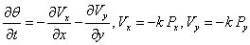
When dealing with porous solids, a fluid as well as a solid description of motion must be incorporated into the governing Equations of the poroelastic structure. In the poroelastic studies performed, Darcy's Law was used to describe the fluid flow through the porous media which was combined with a continuity Equation and the Equations for the solid structure displacement in order to completely describe the media. Eqs. (16) and (16) describe the displacement of a two-dimensional solid matrix in Cartesian coordinates (α, β) (Biot 1941). Eq. (19) relates the fluid pore pressure to the volumetric strain of the cell matrix (epsilson). G is its complex shear modulus, E the Young's modulus, v is the Poisson's ratio, k represents the permeability of the porous medium, α is the Biot-Willis parameter measuring the ratio of the displaced water volume to the volume change of the medium; α is usually equal to unity for a saturated medium. The fluid flow in the extracellular space is proportional to the pressure gradients, Px and Py according to Darcy's law. Eq. (18) is a dynamic continuity Equations accounting for fluid accumulation, theta (Bear and Bachmat 1990; Dullien 1979).

Equation 16

Equation 18

Equation 19

In the studies of the fluid-tissue interactions in the brain presented in this paper, both linear elastic and poroelastic media were used to describe the solid material.

Numerical Method

In this study, analysis was performed using the Finite Elements Method (FEM). FEM is based on the weighted residual method (WRM), a global approach to the evaluation of the residual Equations. Details and additional references about the FEM are given below where the reader can find a detailed explanation of the FE methodology (Xenos and Linninger 2004).

The Method of Weighted Residuals (MWR)

The method of weighted residuals (MWR) is an approximation technique for solving differential Equations. In MWR, a form of the global solution is assumed and then the weights are adjusted to obtain the global fit to the exact solution. The approximating function should satisfy both the essential and natural boundary conditions specified in the problem (Xenos and Linninger 2004; Somayaji 2005). If M is a differential operator acting on a function u to give a function p in Equation 20.

Equation 20

In MWR, u is approximated by a linear combination of trial functions as demonstrated by Equation 21.

Equation 21

If the exact solution u in Equation (20) is approximated by the function in Equation (21) the result of the operation of the differential operator D on u is not p(x) and an error or residual is produced, defined in Equation 22.

Equation 22

The idea in MWR is to force the residual average to zero in the domain, as shown in Equation 23.

Equation 23

In Equation (23), W(xi) are called the weight functions and are equal to the number of unknown constants in u. The result is a set of n algebraic Equations for the unknown constants ai. The choice of the weighting function in Equation (23) determines the type of the weighted residual method (WRM) that include the collocation method, sub-domain method, least squares method, galerkin method, and method of moments.

The Finite Element Method

Steps involved in the finite element analysis of a typical problem include initial discretization of the physical domain into a collection of sub domains called elements. A finite element mesh of the selected elements is then constructed. The nodes and elements are then numbered (Fig. 1) and the geometric properties (e.g. coordinates and cross sectional areas) needed for the problem are generated. Element Equations for all typical elements in the mesh are then derived and the variational formulation of the given differential Equation over the typical element constructed. The element stiffness matrices are then assembled in order to obtain the global stiffness matrix (Equations of the whole problem). The continuity conditions among the primary variables that include relationship between local and global degrees of freedom and element connectivity at nodal points by relating the global nodes to the local nodes are then identified. The boundary conditions are then applied and the assembled system is of the form Ax = b is solved by a linear algebra solver to obtain the solution vector xT. Finally, post-processing is performed in order to view the results (e.g. velocity field, stress on the solid, etc.)

Strong Form

The governing differential Equation with the boundary conditions (Dirichlet or Neumann) is called the strong form or the strong statement and is the conventional form of the differential Equation. The solution obtained by solving the strong statement is exact.

Weak Form

The finite element method is a technique for constructing approximation functions required in an element type application of any variational method. It is required to study the weighted integral formulation and the weak formulation of differential Equations. Since the MWR is an approximate method based on weighted residual method and the differentiation is distributed between the approximate solution Cn and the weight function w, the resulting integral form will require weaker continuity conditions on Cj and hence the weighted integral statement is called weak form. The advantages in using the weak formulation are twofold. First, it requires weaker continuity on the dependent variable and often results in a symmetric set of algebraic conditions in the coefficients. Second, the natural boundary conditions of the problem are naturally included in the weak form and therefore the approximate solution CN is required to satisfy only the essential boundary conditions. These two features of the weak form play an important role in the finite element modeling of the problem.

Areas of Investigation

In this paper, three main case studies were examined involving fluid-structure interactions in the brain: the first was the ventricular distension observed during hydrocephalus, the second, the poroelastic properties of the brain and its effect on brain deformation, and the third, the dynamics of CSF flow through the intracranial compartment. A separate computational simulation was created for each of these three areas of investigation.

Numerical Computational Parameters. First Model:

In the first study, a linear elastic solid was used to represent the solid parenchyma and a pressure was applied on the parenchyma from the ventricles and SAS in order to induce deformation. The initial brain geometry was created based on the dimensions of a horizontal brain slice (Fig 2). The computational mesh consisted of a two-dimensional linear elastic body comprised of two element groups – an inner group representing the white matter and an outer group representing the gray matter (Fig. 3). Normal stiffness values of the brain have been experimentally recorded between 10 and 100 kPa however there is evidence that a decrease in brain tissue elasticity accompanies hydrocephalus (Pena et al. 2002). In order to incorporate this reduction in tissue elasticity, the elastic moduli of 1 kPa and 5 kPa were assigned for white and gray matter respectively. A Poisson's ratio of 0.3 was also assumed. The brain geometry used as well as the material properties assigned were aimed to reproduce the results achieved in previous studies (Pena et al. 2002). The medial edges of the brain slice were then fixed to prevent translation and rotation from occurring at those sites. The magnitude of the pressure difference between the ventricular/subarachnoid spaces and the parenchyma was used in our model since an absolute pressure could not be assigned within the parenchyma using our method. Evidence suggests that under hydrocephalic conditions, the parenchyma acts as a CSF sink indicating a reduced fluid pressure in the parenchyma (Pena et al. 2002). In order to simulate these conditions, a slightly elevated pressure was applied in the SAS and ventricles of 233 and 333 Pa respectively. Recent experiments suggest that no transmural pressure gradients across the parenchyma greater than 133-167 Pa exist (Linninger et al. 2004). Because of this, the 333 Pa pressure applied within the ventricles was only slightly higher than the pressure of 233 Pa applied in the SAS.

Second Model

We then repeated the previous study on a poroelastic medium and incorporated a fluid-filled domain in the ventricle. The same brain slice geometry was again used to generate a geometric grid, but the parenchyma was instead represented as a biphasic poroelastic material (Biot 1941). As before, the solid porous structure was divided into two element groups representing white and gray matter and the same Young's moduli and Poisson's ratio were applied to each tissue type. Additional properties of porosity and permeability were assigned to each of the tissue groups. A porosity of 0.2 for gray matter and 0.4 for white matter was used as well as a permeability of 1015 m-2 and 1012m-2 for gray and white matter respectively (Fig. 4) (Linninger et al. 2005). The same pressure conditions were applied within the ventricles (acting inward on the solid walls of the parenchyma) and the medial edges of the slice were again fixed. Additionally, a wall condition was applied to the bottom edges of the slice to prevent fluid flow across these edges. In the fluid portion of the model, the ventricles, SAS, and pores within the parenchyma were filled with a constant fluid with viscosity of 0.001003 kg/m s and a density of 1000 kg/m3 in order to simulate the water-like material properties of CSF. The medial edges of the SAS and ventricles were left free to allow fluid flux across these boundaries. In both the solid and fluid model, fluid-structure interaction (FSI) boundaries were applied at all interfaces between solid and fluid domains.

Third Model

In the final computational model, the fluid and solid portions of the brain were reconstructed in separate two-dimensional computational meshes from an MRI image of a sagittal slice of the brain. The solid walls of the intracranial vault were fixed in the solid model to prevent any form of translation or deformation from occurring along these walls. The parenchyma was modeled as a linear elastic body around which CSF was allowed to flow. For the purpose of simplification, no differentiation was made between white and gray matter within the parenchyma and an Elastic modulus of 10 kPa, representative of the normal stiffness values of brain tissue, was applied to the brain tissue (Pena et al. 2002). A Poisson's ratio of 0.45 was also assumed in order to mimic the near-incompressibility of the human brain. It is known that the choroid plexus produces CSF at the rate of 0.35 ml/min. For this reason a constant fluid flux of 0.35 ml/min from the upper surface of the choroid plexus into the lateral ventricles was modeled. Fluid was permitted to flow through the ventricular system and the SAS, as well as exit and enter the spinal SAS. In order to mimic the effect of the pulsatile expansion of the vasculature bed within the brain, a consolidated arterial system was incorporated into the model in the form of an expansible linear vessel within the parenchyma (Fig. 5). A prescribed outward displacement of 1.125 mm maximum was applied to the length of the vessel walls. The expansion of the vasculature system was also implied through an inward displacement of 3 mm maximum of the external wall of the intracranial space in the prepontine region in order to address the effects of the expansion of the basal artery in that region. Finally, a slight expansion of the choroid plexus was also created by applying an outward displacement of 0.43 mm maximum on the upper and lower solid walls. In order to accurately simulate the pulsatile nature of the vascular expansion, all of the described displacements were applied as cardiac pulse (Fig. 6) described by Equation 24.

Equation 24

The interior walls of the ventricular system were allowed to deform while the exterior surface of the parenchyma and the aqueducts were fixed preventing translation (Fig. 5).

RESULTS

Hydrocephalic-Like Ventricular Distension Observed in First and Second Models

In both the linear-elastic and poroelastic simulations of brain deformation during hydrocephalus, ventricular expansion in accordance with clinical and experimental observations was observed. Although a slight compression of the cerebral surface was sustained due to the pressure acting from the SAS, in both cases a much more substantial deformation was observed in the ventricles. The expansion of the ventricles was predominantly directed laterally and produced a diminishing of the horns of the lateral ventricles, creating a rounder enlarged ventricle (Figs. 7, 8). The maximum displacement observed in both cases was directed laterally in the ventricles in the region of the thalamus. The maximum displacement in both cases was observed in the center of the outermost edge of the lateral ventricles with a value of 6.748 mm in both cases. The similarities of these displacements indicate that very little difference in the deformations of the linear elastic and poroelastic cases exists. The maximum stress observed in both cases occurred on the horns of the ventricular walls (Figs. 9, 10).

Fig 1: Node and element definitions on a finite element mesh.

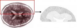
Fig 2: Diagram of the biological geometry used to create the computational mesh. One hemisphere of a horizontal brain slice was broken down into the domains of the ventricle, white matter, gray matter, and SAS.

Fig 3: The computational mesh for the linear elastic case study composed of gray and white matter regions.

Fig 4: The computational mesh for the fluid model of the poroelastic case study composed of gray and white matter regions as well as cerebrospinal fluid regions.

Cerebrospinal Fluid Motion Observed in Second (Poroelastic) Model

In the poroelastic simulation, the pressure applied to the ventricular surface induced a flow of cerebrospinal fluid out of the ventricles, through the parenchyma, and into the cerebral SAS as evidenced by the directional plot of fluid velocity. It was noted that the displaced fluid exited laterally through the ventricles, traveled through the white matter and gray matter, and exited into the cerebral SAS. However, a recirculation directed back medially occurred as the flow progressed through the white matter, presumably due to the lower porosity of the gray matter impeding the fluid flow from the higher porosity white matter into the less porous gray matter. The maximum velocity of 0.3374 mm/s occurred in along the center of the lateral edge of the ventricle while the lowest velocity areas were in the outer portions of the cerebral SAS (Fig. 11).

Fig 5: Computational mesh for the solid model showing prescribed and deformable boundary conditions.

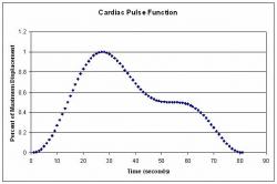
Fig 6: Cardiac function used to describe assigned displacements which was extracted from experimental data of the cardiac pulse, the equations used can be shown in equation (24).

Fig 7: Linear elastic model showing displacement magnitude which was greatest in the center (red color regions) of the lateral edge of the ventricular wall.

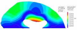
Fig 8: Poroelastic case study solid model showing displacement magnitude. The maximum solid displacement (red color regions) occurred in the center of the lateral edge of the ventricular wall.

Simulated Vascular Expansion Drove Tissue Expansion and CSF Circulation in Third Model

When the dynamics of the simulated vascular expansion were observed, it was found that the simulated arterial system effectively caused an expansion of the solid parenchyma. According to our model, this caused compression of the lateral ventricles which, when coupled with the expansion of the choroid plexus, created a significant decrease in the ventricular volume. The displacement magnitude during systole in the ventricular region was largest on the upper surface of the lateral ventricle (which was compressed downwards) (Fig 12). The maximum systolic effective stress occurred at the walls of the anterior and posterior horns of the lateral ventricles (Fig. 13). During late diastole, a slight outward displacement of the ventricles was also observed (Fig. 14, 15).

During systole, fluid exited the ventricles and flowed down the aqueduct of Sylvius and foramens of Luscke and Magendie, finally being forced down into the spinal SAS. Velocity maxima were observed in the aqueduct of Sylvius and in the prepontine region during systole. Also during systole, a velocity maximum of 0.0043875 m/s was observed in the aqueduct of Sylvius (Fig. 16). As the simulation entered into diastole, a reversal of flow was observed causing fluid to enter the intracranial vault from the spinal SAS and flow upwards into the cerebral SAS and through the ventricular system into the lateral ventricles (Fig 16). The maximum velocity during diastole also occurred in the aqueduct of Sylvius, although nearer the entrance to the 3rd ventricles than the systolic maximum, and was directed upwards into the ventricles at 0.00246 m/s (Fig. 16). When smaller fluid velocities were examined, it was also noted that a small reversing flow occurred in the cerebral SAS, circulating dorsally during systole and back ventrally during diastole.

Fig 9: Linear elastic model showing effective stress which was greatest at the edges of the fixed portion of the slice and at the anterior and posterior horns of the lateral ventricles.

Fig 10: Poroelastic case study solid model showing effective stress which was also greatest at the edges of the fixed portion of the slice and at the anterior and posterior horns of the lateral ventricles.

Fig 11: Fluid velocity magnitude plot for the poroelastic case study showing that maximum velocity occurred along the central edge of the lateral ventricle and a very substantially reduced fluid velocity was present within the parenchyma as compared to the ventricles.

Fig. 12: Displacement magnitude during systole surrounding the lateral and 3rd ventricles. The maximum displacement of more than 3.4 mm occurred on the upper surface of the ventricular wall as it was compressed downward by the expanding parenchyma.

DISCUSSION AND CONCLUSIONS

Linear Elastic Case Study.

In the linear elastic model of hydrocephalus, it was shown that a deformation nearly identical to the ventricular distension observed during hydrocephalus could be effectively produced through the application of a very minimal transmural pressure gradient (100 Pa) – so small as to be below the smallest detectable pressure difference (133-167 Pa). These findings support recent studies that have negated the existence of the large pressure difference between the ventricular system and the SAS that was previously thought to be present in hydrocephalus (Linninger et al. 2005). The lateral expansion of the ventricles and the decrease in prominence of the anterior and posterior horns were much like the expansion observed in MRI images of hydrocephalus. Overall, this case study demonstrates that a 100 Pa trans-parenchymal pressure gradient is sufficient to produce hydrocephalic-like ventricular distension, validating previous work which claimed that little or no trans-parenchymal pressure gradient existed in communicating hydrocephalus (Linninger et al. 2005).

Fig. 13: The effective stress during systole was largest in the expanding choroid plexus and on the walls of the anterior and posterior horns of the lateral ventricles, approaching 533.4 N/m2.

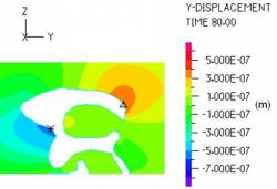
Fig. 14: The y-displacement in the ventricular area during late diastole was largest on the posterior horn of the lateral ventricle (0.0004 mm) and anterior edge of the foramen of Monroe (0.0007 mm) indicating that after the prescribed moving boundaries have returned to their original positions, a very slight deformation of the ventricles, presumably due to the CSF velocity, is present.

Fig. 15: The z-displacement in the ventricular area during late diastole indicates that the reversal of flow up into the ventricles during diastole deforms the lateral ventricle wall upwards a maximum distance of about 0.0002mm after the parenchyma has returned to its original size.

Fig. 16: CSF velocity magnitude during systole (left) and diastole (right). The maximum velocity achieved during systole is marked in the aqueduct of sylvius and was directed downward towards the spinal SAS. The maximum velocity achieved during diastole is also marked in the aqueduct of sylvius and was directed upward into the third and lateral ventricles

Poroelastic Case Study

The poroelastic model of hydrocephalus also supported the negation of a large transmural pressure gradient in hydrocephalus, showing nearly identical deformation to that observed in the linear elastic model when subjected to identical pressures. In addition, the fluid flow into the parenchyma induced by the applied pressure provided direct evidence that deformations of the brain tissue may cause a shift in brain water content. Overall, this case study showed that the application of pressure to the solid brain could induce a fluid flow within the porous brain, suggesting a shift in brain water content may occur under such conditions, thus changing the effective properties of the brain tissue.

Simulation of CSF Flow

Our model of CSF flow through the intracranial compartment effectively simulates the flow fields obtained through experimental MRI flow imaging - including a reversal of flow during diastole - without the application of an arbitrary CSF sink or negative flux within the ventricles. By simulating the expansion of the parenchyma and choroid plexus due to pulsatile blood flow through the cerebral vascular bed, a pulsatile change in the volume of the lateral ventricle, similar to what has been observed experimentally, was created (Zhu et al. 2006). Most importantly, this final case study validated the brain motion hypothesis, demonstrating that the vasculature system could induce a net motion of the solid brain which in turn induced the pulsatile CSF flow previously observed using MRI.

Proposed Sequence of Events

During systole, expansion of brain vasculature causes an expansion of the parenchyma. This results in an inwardly directed displacement of the ventricular walls. In addition, simultaneous vasculature expansion within the choroid plexus causes it to expand, forcing CSF outwards into the compressing ventricular walls. This nested compression of the walls and expansion of the choroid plexus causes a decrease in the overall volume of the lateral ventricles as well as a transient increase in the pressure within the ventricles, causing CSF to be forced down its pressure gradient and out of the ventricular system, achieving a maximal velocity in the narrow aqueduct of Sylvius before exiting the intracranial vault into the spinal SAS. Likewise, in the prepontine region, the systolic expansion of the basal artery causes an inward displacement of the walls of the adjacent fluid pathways, again transiently decreasing the available volume for CSF to occupy and forcing the fluid down into the spinal SAS.

As the cardiac cycle progresses, the elasticity of the vasculature system returns the vessels to their pre-systolic volume, causing a contraction of the parenchyma and subsequent increase in ventricular volume as the walls retract outwardly and the choroid plexus returns to its original size. This ventricular expansion causes a transient decrease in pressure causing CSF to again flow down its pressure gradient, this time upwards from the spinal SAS back into the ventricular system. Simultaneously, the diastolic retraction of the walls of the prepontine area causes a similar increase in volume in that region, instigating a similar reversal of flow from the spinal SAS up into the prepontine and cerebral SAS regions.

Implications of Findings

In this study it was shown that despite a constant positive flux of CSF into the ventricles, a change in ventricular volume due to dynamics of the vasculature system was independently able to cause a reversal of CSF flow as is observed in MRI data. This simulation demonstrates that CSF dynamics are in fact a function not only of the brain geometry and rate of CSF production/reabsorption, but also of the fluid-structure interactions between CSF, the solid brain, and the vasculature system. This finding validates the brain motion hypothesis which states that the cerebral blood flow causes motion of the solid brain which in turn drives the pulsatile CSF flow (Greitz 2006; Enzman and Pelc 1992). Thus, when pathological conditions such as hydrocephalus are considered, it is no longer sufficient to consider an imbalance in CSF production and reabsorption rates alone. The prominent role the vasculature system and mechanical properties of the brain tissue play in the dynamics of normal CSF flow suggest that they too be implicated as causes of conditions of abnormal flow such as those observed during hydrocephalus.

In all of the case studies is was found that cerebrospinal fluid-tissue interactions are a primary factor in the determination of intracranial dynamics and thus an important consideration when attempting to better understand and appropriate treatment for cerebral diseases such as hydrocephalus.

Future Directions

In order to more clearly determine the role that the vasculature system and the mechanical properties of the brain tissue play in creating a disease state, it is recommended that future studies investigate pathological-like CSF flow patterns and tissue deformations through the application of parameters consistent with known possible confounders with cerebral disease (e.g. decreased brain tissue compliance).

REFERENCES

ADINA R & D Inc, (ADINA), http://www.adina.com/.

Bathe, Klaus-Jurgen (1975) Finite Element Formulations for Large Deformation Dynamic Analysis. International Journal for Numerical Methods in Engineering, 9: 353-386.

Bear J., Bachmat Y. (1990) Introduction to Modeling of Transport Phenomena in Porous Media, ed. J. Bear. Vol. 4, Dordrecht, Kluwer Academic Publishers.

Bering, Edgar A. (1961) Circulation of the Cerebrospinal Fluid.

Biot, M.A. (1941) General Theory of Three-Dimensional Consolidation. Journal of Applied Physics 12: 155-164.

Chou P.C. and Pagano N.J. (1992) Elasticity: Tensor, Dyadic, and Engineering Approaches, Dover Publications, Inc., New York.

Du Boulay, G. H. (1966) Pulsatile Movements in the CSF Pathways. British Journal of Radiology 39: 255-262.

Du Boulay, G, J O'connell, J Currie, Thea Bostick, and Pamela Verity (1972) Further Investigations on Pulsatile Movements in the Cerebrospinal Fluid Pathways. Acta Radiologica Diagnosis 13: 496-521.

Dullien F.A.L. (1979) Porous Media Fluid Transport and Pore Structure. Academic Press, INC.

Enzmann, D. R., N. J. Pelc (1992) Brain motion: measurement with phase-contrast MR imaging. Radiology 185: 653-660.

Greitz, Dan (2004) Radiological assessment of hydrocephalus: new theories and implications for therapy. Neurosurgery Reveiew 27: 145-165.

Hakim, Salomon, Jose G. Venegas, and John D. Burton (1976) The Physics of the Cranial Cavity, Hydrocephalus and Normal Pressure Hydrocephalus: Mechanical Interpretation and Mathematical Model. Surgical Neurology 5: 187-210.

Linninger, Andreas A., Cristian Tsakiris, David C. Zhu, Michalis Xenos, Peter Roycewicz, Zachary Danziger, and Richard Penn (2005) Pulsatile Cerebrospinal Fluid Dynamics in the Human Brain. IEEE Transactions on Biomedical Engineering 52: 557-565.

Linninger, Andreas A., Michalis Xenos, David C. Zhu, Mahadevabharath R. Somayaji, Srinivasa Kondapelli, and Richard Penn (2007) Cerebrospinal Fluid Flow in the Normal and Hydrocephalic Human Brain. IEEE Transaction on Biomedical Engineering 54(2): 291-302.

Linninger, Andreas A., Michalis Xenos, Srinivasa Kondapalli, and Mahadevabharath R. Somayaji (2005) Mimics Image Reconstruction for Computer-Assisted Brain Analysis. Mimics. .

Linninger, Andreas A., M.B.R Somayaji, M. Xenos and S. Kondapalli (2004) Drug Delivery in the Human Brain. Foundations of Systems and Biology Engineering (FOSBE), Univ. of California, Santa Barbara, August 7-10.

Love, A.E.H., (1944), A treatise on the mathematical theory of elasticity, 4th ed., New York: Dover Publications.

Naidich, Thomas P., Nolan R. Altman, and Sergio M. Gonzalez-Arias (1993) Phase Contrast Cine Magnetic Resonance Imaging: Normal Cerebrospinal Fluid Oscillation and Applications to Hydrocephalus. Neurosurgery Clinics of North America 4: 677-705.

Patwardhan, Ravish V., and Anil Nanda (2005) Implanted Ventricular Shunts in the United States: the Billion-Dollar-a-Year Cost of Hydrocephalus Treatment. Neurosurgery 56: 139-145.

Pena, Alonso, Neil G. Harris, Malcolm D. Bolton, Marek Czosnyka, and John D. Pickard (2002) Finite Element Modeling of Progressive Ventricular Enlargement in Communicating Hydrocephalus Acta Neurochir. Suppl. 81: 59-63.

Rekate, H L., S Erwood, J A. Brodkey, and et al. (1985) Etiology of Ventriculomegaly in Choroids Plexus Papiloma. Pediat. Neuroscience 12: 196-201.

Schlichting H.(1979) Boundary-Layer theory, 7th Ed., McGraw-Hill, New York.

Somayaji, M.B.R (2005) Numerical Solution of Two-Dimensional Steady Diffusion Equations Using Finite Element Method. UIC–LPPD-050705.

Xenos M. and Linninger A.A. (2004) Finite Elements Method. UIC-LPPD-0125056.

Zhu, DC., M. Xenos, A.A. Linninger, and R.D. Penn (2006) Dynamics of Lateral Ventricle and Cerebrospinal Fluid in Normal and Hydrocephalic Brains. Journal of Magnetic Resonance Imaging 24: 756-770.