

Author: Jessica L. Williamson, Hakeem M. Oluseyi, Natalie Roe
Institution: The University of Alabama - Huntsville
Date: July 2007
ABSTRACT
Dark energy, which is believed to be a cosmic energy density that is gravitationally repulsive and does not appear to cluster in galaxies, has been invoked to account for the recent measurement that the rate of the universe's expansion is accelerating. To better understand these phenomena, scientists utilize type Ia supernovae as calibrated candles. Lawrence Berkeley National Laboratory (LBNL) is developing the Supernova Acceleration Probe (SNAP), a space-based telescope that will be used to identify and measure supernovae. The SNAP focal plane will consist of an innovative camera that integrates two cutting-edge imaging sensor systems, one of which is the LBNL high purity charged-coupled device (CCD) for the visible light range. We report on the development of a novel technique for extending the spatial and photometric fidelity performance of the LBNL CCDs. In this study, results were obtained from measurements using a 10.5 µm pixel pitch, 1.4k×1.4k format, p channel CCD fabricated on high-resistivity silicon at LBNL. The fully depleted device is 300 µm thick and backside illuminated. Measurements of the device's transverse diffusion of charge carriers, and pixel to pixel uniformity are reported. Also presented are preliminary results from the first implementation of CCD Phase Dithering, a novel technique for achieving sub-pixel spatial resolution in under-sampled, pixelated image data as will be obtained by the SNAP satellite.
INTRODUCTION
Since Hubble's discovery in the early 20th Century that the universe is expanding, researchers believed that the rate of expansion was decreasing due to the mutual gravitational attraction of the universe's matter. For about a decade, astronomers at the Lawrence Berkeley National Laboratory (LBNL) attempted to measure the deceleration rate. This effort led to the shocking discovery in 1998 that the rate of the universe's expansion is actually accelerating [1]. An unknown energy, termed "dark energy," has been invoked to account for the universe's acceleration. The simplest model for dark energy describes a cosmic energy density which permeates all space, is gravitationally repulsive, and does not cluster in galaxies. Precision measurements of the universe's dynamics and the determination of the nature of the dark energy that accelerates its expansion have now been identified as among the most important scientific priorities of our day [2,3].
Two methods for elucidating the nature of dark energy include measurement of the universe's dynamics and measurement of the universe's contents. Type Ia Supernovae (SNe Ia) are very useful tools for measuring the dynamics of the universe. They are generated when a white dwarf star in a binary system accretes mass from its companion, approaches the Chandrasekhar limit (i.e., the maximum mass for a white dwarf), and explodes. The peak luminosities of all SNe Ia are similar because their masses at the time of explosion are all nearly the same. SNe Ia are also the brightest type of supernovae, allowing them to be seen over cosmic distances. Moreover, SNe Ia are easily distinguished from other types of exploding stars due to their unique spectral signature. With these characteristics, SNe Ia become bright, easily identifiable, astronomical objects of known luminosity, or a standard candle. Because their intrinsic luminosities are known, one may determine the distance to a SNe Ia by carefully measuring its apparent luminosity. Since light travels at a well-known (but finite) speed, measurement of the distance to a SN Ia is equivalently a measurement of the time that has surpassed since the light was emitted from the SN Ia. Likewise, the spectral features that allow us to identify SNe Ia also allow us to make an additional measurement of the universe's dynamics. It turns out that as light travels through the expanding space of the universe, its wavelength is stretched by the exact amount that space expanded as the photon traveled through the medium. Thus, measurement of the apparent luminosity and spectrum of a SN Ia provides a direct measure of the size of the universe versus time. This technique is exactly that used by LBNL researchers to discover the dark energy (Figure 1).

Figure 1: Light travels through the expanding space of the universe, its wavelength is stretched by the exact amount that space has expanded. Thus, while it is traveling measurement of the apparent luminosity and spectrum of a SN Ia provides a direct measure of the size of the universe versus time. This technique is exactly that used by LBL researchers to discover dark energy; this figure shows their data
An additional method for elucidating dark energy involves measuring the contents of the universe. A powerful new technique for performing this task is called gravitational weak lensing. Gradients in the gravitational potentials of foreground matter induce a small but measurable tangential elongation, or "shear", in the images of background galaxies (Figure 2). The detections and mapping of this weak lensing signal is one of the most exciting and challenging areas of precision cosmology. The variation of this cosmic shear as a function of angular scale is the most direct constraint on both the amount and statistical distribution of dark matter, which constitutes the vast majority of all attractively gravitating matter in the universe [4]. Also, the statistical pattern of these distortions is sensitive to the cosmic expansion history and thus to the dark energy.

Figure 2: In weak lensing, shapes of galaxies are measured. Large-N statistics extract lensing influence ("shear") from intrinsic noise. Dominant noise source is the (random) intrinsic shape of galaxies
Accurate, high-precision measurements of the luminosities of SNe Ia and the shapes of galaxies at the necessary levels require novel, cutting-edge technologies. To achieve these scientific goals, researchers at the Lawrence Berkeley National Laboratory (LBNL) are in the process of developing the Supernova Acceleration Probe satellite (SNAP). SNAP is a 2-meter space-based telescope scheduled to launch in 2013 (Figure 3), which will undertake measurements of SNe Ia light curves and spectra, and will also generate weak lensing maps over large regions of the sky. Performing these measurements at there necessary precision places stringent requirements on SNAP detector technologies.

Figure 3: Supernova Acceleration Probe satellite (SNAP) is a 2-meter space-based telescope scheduled to launch in 2013
SNAP's imager camera will be integrated with two imaging sensor systems: the LBNL high-resistivity charged coupled devices (CCDs) for the visible and HgCdTe sensors for the near infrared. Our work here is focused on characterizing the spatial fidelity performance of the LBNL CCD and the development of novel observational techniques utilizing the LBNL CCD (Figure 4). LBNL CCDs offer several advantages over other types. These include sensitivity to a wider range of light energies and wavelengths [5,6], improved radiation tolerance (a requirement for reliable and robust operation in space), [7,8], and improved control over spatial information [9,10]. Figure 5 shows the effect of lateral charge diffusion in a back-illuminated CCD. Light creates a bundle of charges near the CCD's backside, which spread prior to being collected in the frontside CCD circuitry. In order to perform weak lensing science, it is necessary to characterize and control the amount of spreading caused by diffusion. Moreover, pixel to pixel and intrapixel response variations can limit the accuracy of photometric and spatial measurements.

Figure 4: The advantages of the LBNL high-resistivity charged coupled devices (CCDs). Includes: sensitivity to a wider range of light energies and wavelengths, improved radiation tolerance (a requirement for reliable and robust operation in space), and improved control over spatial information
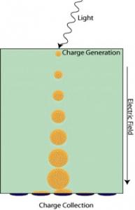
Figure 5: Shows the effect of lateral charge diffusion in a back-illuminated CCD
This report describes measurements of LBNL CCD properties including charge diffusion and, pixel to pixel variations. The feasibility of a novel new technique which we have coined "CCD Phase Dithering," designed to achieve sub-pixel resolution from under-sampled image data, is tested for the first time. The successful development of this technique has the potential for substantially improving the observational efficiency and the spatial and photometric fidelity of the SNAP satellite.
MATERIALS AND METHODS
To perform our characterization experiments, the CCD is mounted inside an Infrared Laboratories ND-8 3206 liquid nitrogen dewar, a vessel designed to provide very good thermal insulation and maintain a high vacuum. The CCD is operated at very cold temperatures (133 K) to minimize unwanted charges (the dark current) generated by thermal fluctuations within the silicon lattice, which are independent of any light signal. Dark current effects are reduced significantly at such low temperatures. The ultra-high vacuum (10-5 10-7) is necessary to draw out vapors that would condense on the CCD when it is cooled, thereby short-circuiting and destroying the device.
The CCD is run by a computer-controlled Leach controller. The Leach controller is a dual readout controller from Astronomical Research Cameras, Inc. It has several boards which help to operate and readout the CCD. The utility board, based on a Motorola DSP 56001, controls the exposure timing and shutter operation. The timing board, based on a Motorola DSP 56002FC66, generates digital timing signals to control other circuit boards and communicates with the host computer. The video board processes and digitizes the video output from the CCD, and supplies digitally programmable DC bias voltages to the CCD. The clock driver board provides analog voltage levels from +10V to 10V for the clock signals.
To perform characterization experiments, the CCD is illuminated by a light source external to the dewar. Light from a high-intensity General Electric bulb passes through a filter before it is focused onto a fiber optic cable bundle by means of a convex lens. A centering assembly holds the fiber optic cable in place inside a brass tube. The light illuminates a 10 μm pinhole, passes through a tube, and is collimated by a tube lens. The collimated light is then focused to about 1 μm on the CCD by a microscope objective, with a working distance of 34 mm Figure 6 shows our experimental setup.
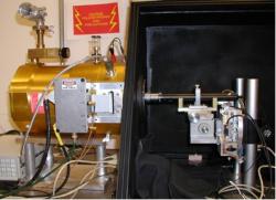
Figure 6: The apparatus shown is the pinhole projector. To perform characterization experiments, the CCD is illuminated by a light source external to the dewar. Light from a high-intensity General Electric bulb passes through a filter before it is focused onto a fiber optic cable bundle by means of a convex lens. A centering assembly holds the fiber optic cable in place inside a brass tube. The light illuminates a 10 μm pinhole, passes through a tube, and is collimated by a tube lens. The collimated light is then focused to about 1 μm on the CCD by a microscope objective, with a working distance of 34 mm
Several techniques are used to characterize the performance of the LBNL CCD. These include: the virtual knife-scan technique, which measures lateral charge diffusion; the spot integration technique, which measures beam stability, a source of measurement uncertainty; and the pixel signal technique, which measures pixel to pixel uniformity.
The virtual knife-edge experiment is derived from the real knife edge experiment, a commonly used tool for determining the diameter of a beam. In a real knife-edge experiment, an obstructing device such as a razor blade is placed between a light beam and a detector, which outputs a voltage or current proportional to the light incident upon it. The projected beam is scanned across the knife edge in several small steps. At each step, the beam is incrementally blocked by the knife edge. The light intensity at the detector is measured at each step. The distance covered from the beginning of the attenuation of the beam signal to the complete attenuation of the signal provides information on the beam diameter. The exact form of the beam intensity fall-off with distance provides information on the beam profile. The virtual knife-edge experiment is similar; in this study, the CCD is used as the detector. Unlike the earlier detector, the CCD provides spatial information but suffers from charge diffusion; also, a physical obstruction is not used to block the light. Instead, a region of the CCD, called the integration square, is arbitrarily defined. The beam is stepped across the CCD and an image is obtained at each step (Figure 7). Later, we sum the light in the integration square for the series of images. The scan is set up so that the spot steps out of the integration square, attenuating the integrated intensity in the square over the course of the scan. The edge of the square has the same function as the edge of the razor blade in a standard knife-edge experiment. By comparing the size of the beam determined in the two approaches, we determine the amount of lateral diffusion in the CCD.
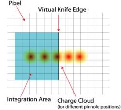
Figure 7: Illustrates the virtual knife edge scan technique
The spot integration technique is used to measure the beam stability. Instead of maintaining an integration square in a defined region of the CCD, we integrate the spot signal at each step with the spot always in the center of the integration region. Any changes in the integrated signal can be attributed to the convolution of the beam signal and the CCD response. To de-convolve these two contributions, we measure the uniformity from pixel to pixel. In this case, we define a row of target pixels. As the scan moves across the pixels we measure the signal in each pixel as a function of the beam position. This technique will elucidate any non uniformity of pixel response.
Intra-pixel variations are measured by scanning the beam across the CCD by fractions of a pixel at a time, therefore achieving multiple pointings within a single pixel, a process known as dithering (Figure 8). Note that each pixel in a CCD is defined by three MOS transistor gates on the front-side of the CCD. The signal of level each pixel in an image is determined by photo-generated charges collected under one of the three gates with pixels separated by two gates. In a dithered scan, each time the beam is realigned, light falls on different parts of the CCD but within the same pixel region. The number of charge carriers collected in each pixel is counted and recorded, providing insight into the intensity of light hitting that pixel. Thus, in a dithered scan each exposure is slightly different (Figures 9a,b). The set of images provides enough data to form a superimage (Figure 10), which will possess spatial resolution superior to the individual images from which it was constructed. Likewise, by fitting a Gaussian to the beam signal in the individual images that comprise the dithered scan, we can determine response variations within an individual pixel.

Figure 8: 9-point dither pattern

Figure 9a: Move an image across the CCD fractions of a pixel at a time and take a picture

Figure 9b: Each exposure is slightly different

Figure 10: After all the dithered images are collected they are reconstructed to form a super-image
Finally, we wish to test the concept and feasibility of a new technique that we have devised called CCD Phase Dithering. Our new phase dithering technique is designed to achieve the same performance as a standard dithering technique but with many fewer pointings. Typically, the image that is obtained from a CCD is given by the convolution of the original object being imaged, O(x,y), with the point spread function of the optics which focus the light upon the CCD, P(x,y), and the spatial response of each CCD pixel Π(x,y).
In a standard dithering experiment, P(x,y) and Π(x,y) are each held constant while O(x,y) is varied. In our new phase dithering technique, P(x,y) and O(x,y) are held constant while Π(x,y) is varied. Figures 11 and 12 illustrate the equivalence of the two approaches. In Figure 11, we place a 10,000 electron signal on phase-two of a CCD which utilizes phase-one as its collection phase. We see that the charges are distributed asymmetrically between the two adjacent pixels. The number of charge carriers collected under the collection phases of each pixel depend on their distances from the original 10,000 electron signal. Next we move the signal to phase-two and phase-three respectively, each time generating a redistribution of the carriers under the two adjacent pixels. In Figure 12, we keep the signal stationary over phase-three but now permute the collection phase in each of two subsequent images. Note that the same distribution of charges is generated within the adjacent pixels. By using this technique, we are able to achieve the effect of nine pointings with only three pointings. The internal electronics of the CCD are able to mimic the effect of the other six pointings. This technique will reduce time between images and reduce the need for multiple high-precision pointings of a large telescope. Note, however, that this technique only works in one spatial direction.

Figure 11: During standard dithering every time the telescope is realigned charges fall on different parts of the CCD

Figure 12: Phase dithering generates the same results by changing the gate under which the charge is collected
To implement the phase dithering technique, we illuminate the CCD with the 1 m spot with three pointings per pixel. At each pointing three images are taken with the CCD utilizing a different collection phase each time. The images will be recombined to form a superimage.
RESULTS
The knife-scan technique results can be seen in Figure 13. This shows that the charge is constant while focused in the integrated region of the CCD. The change starts to decrease as the spot is moved out of the integrated region forming a slope in the graph. Then the graph reaches a constant change again when the spot is no longer inside the integrated region. The form of this graph represents an error function, which is shown as a line-fit to the data points. The derivative of the error function is a Gaussian. We have fit a Gaussian curve to this curve; its full width at half maximum, σ(CCD), provides us with the width of the beam as measured by the CCD. Utilizing the intrinsic beam width measured with a real knife-scan technique, σ(CCD), we derive the rms diffusion within the CCD. The measured diffusion is 7.4 µm.
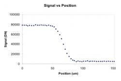
Figure 13a: The signal in an integration square as a projected spot is moved out of the region. The signal level in the region begins to attenuate as the spot leaves the region. Fitting a curve to this data reveals the size and profile of the spot

Figure 13b: This curve represents the inverse derivative of Figure 13a. The dark blue line represents the data while the pink line represents a Gaussian fit to the data. The measured width of the Gaussian is σ= 7.5 μm
Figure 14 shows the results of the beam stability measurement. A cursory examination of this figure suggests that there is a periodic error in the beam stability with a period of about 10 pointings. Each image takes a total of about 30 seconds to integrate and download. The 10 pointing signal, therefore, corresponds to a modulation of the beam stability possessing a period of about five minutes. The total variation observed may be ascertained from Figure 14b. This images shows residuals of the signal as compared to a line fit to the data. The observed variation is ± 2%.
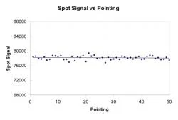
Figure 14a: The spot integration technique is used to measure the beam stability. Instead of maintaining an integration square in a defined region of the CCD, we integrate the spot signal at each step with the spot always in the center of the integration region

Figure 14b: The beam level is measured for a series of spots. The integrated signal is fit to a line and the fit residuals (± 2%) are plotted
The beam stability results impact our ability to determine intra-pixel sensitivity variations. We wish to have a signal stability of less than or equal to 1% to make this measurement. These results suggest we should perhaps consider a different experimental setup, perhaps utilizing a LED.
We wish to determine the uniformity of the pixels. The pixel uniformity data are plotted in Figure 15 to see whether response varies significantly from one pixel to the next. The peak values of the curves vary by ± 2% illustrating that the responses are consistent within each pixel.

Figure 15: Pixel uniformity measurements. Each curve represents a pixel as the spot is scanned across it. The signal is relatively constant as the spot is stepped across the pixels. The observed variations in peak pixel signals are ±2%. This variation is consistent with the variation in the beam signal stability

Figure 16: An illustration of dithering versus phase dithering. (a) this photo is a raw spot image without dithering. (b) this image shows a reconstructed superimage from nine images taken in a 9-point dither pattern. (c) this image shows a reconstructed superimage from nine images taken with only three pointings but with phase dithering to mimic the 9-point dither pattern. Note that the last two images are virtually identical
Figure 16 shows a comparison of normal dithered data with phase-dithered data. From left to right, the first spot is an image of the beam with no dithering. The second spot shows the superimage formed from using the standard dithering technique involving nine independent pointings. The third spot shows the superimage formed from our phase-dithered exposures. The standard dithering and phase-dithering images are virtually indistinguishable. These images clearly illustrate the equivalence of the phase-dithering process to standard dithering.
DISCUSSIONS AND CONCLUSIONS
We have developed a novel technique for extending the spatial and photometric fidelity performance of the LBNL CCDs. The results obtained were measured using a 10.5 μm pixel pitch, 1.4k×1.4k format, p channel CCD fabricated on high-resistively silicon at LBNL. The fully depleted device is 300 µm thick and backside illuminated. Measurements of the device's transverse diffusion of charge carriers was 7.4 μm, pixel to pixel uniformity showed some signal variations, and the intra-pixel uniformity. The first implementation of CCD phase-dithering clearly illustrates the concept and feasibility of CCD phase dithering.
Further research will be conducted to characterize the performance of the device as a function of the gate chosen for collection for phase dithering. Investigation of our current data more thoroughly, and examining the images differences from the two types of dithering techniques, determining intra-pixel variations in sensitivity and psf, and investigating device design modifications to improve phase dithering performance.
ACKNOWLEDGMENTS
This research was conducted at the Lawrence Berkeley National Laboratory. I would like to thank my mentor Dr. Hakeem Oluseyi for enlightening me with his knowledge, for providing me with many opportunities, and for his persistent patience. The completion of this work would not have been possible without the guidance and assistance of the SNAP CCD team and the SCP analysis team. We extend our gratitude and thanks also to Dr. Natalie Roe, Dr. Chris Bebek, Dr. Kyle Dawson, Mr. Armin Karcher, Dr. William Kolbe, Dr. Michael Levi, and Mr. David Rubin. We would also like to thank Mr. Toan Nguyen of The University of Alabama in Huntsville. Lastly, thanks to the Department of Energy and the Office of Science for this wonderful opportunity to participate in the Science Undergraduate Laboratory Internship (SULI) program.
This material is based upon work supported by the National Science Foundation under Grant No. 0449962. Any opinions, findings, and conclusions or recommendations expressed in this material are those of the author(s) and do not necessarily reflect the views of the National Science Foundation. Any opinions, findings, and conclusions or recommendations expressed in this material are those of the author(s) and do not necessarily reflect the views of the National Science Foundation.
REFERENCES
[1] R. Caldwall. Dark Energy. http://physicsweb.org/articles/world/17/5/7.
[2] Dark Energy. http://imagine.gsfc.nasa.gov/docs/science/mysteries_l1/dark_energy.html. [3] Dark Energy Confirmed as Constant Presence. http://msnbc.msn.com/id/4327735/. [4] Dark Energy .http://en.wikipedia.org/wiki/Dark_energy. [5] D. E. Groom, C. J. Bebek, M. Fabricius, A. Karcher, W.F. Kolbe, N. A. Roe, & J. Steckert, "Quantum efficiency characterization of back-illuminated CCDs Part 1: The Quantum Efficiency Machine," in SPIE 6068 (2006). [6] C. J. Bebek, D. E. Groom, S. E. Holland, A. Karchar, W. F. Kolbe, M. E. Levi, N. P. Palaio, B. T. Turko, M. C. Uslenghi, M. T. Wagner, G. Wang "Proton radiation damage in high-resistivity n-type silicon CCDs," LBNL-49933 , SPIE 4669, 161-171 (2002). [7] Jessamyn A. Fairfield, D. E. Groom, S. J. Bailey, C. J. Bebek, S. E. Holland, A. Karcher, W. F. Kolbe, W. Lorenzon, & N. A. Roe, "Improved spatial resolution in thick, fully depleted CCDs with enhanced red sensitivity," submitted to IEEE Trans. Nucl. Sci., (April 2006). [8] Jessamyn A. Fairfield "Improved spatial resolution in thick, fully depleted CCDs with enhanced red sensitivity," in Proc. IEEE Nucl. Symp. Med. Imaging Conf., Nov. 2005. [9] A. Karcher, C.J. Bebek, W. F. Kolbe, D. Maurath, V. Prasad, M. Uslenghi, M. Wagner, "Measurement of Lateral Charge Diffusion in Thick, Fully Depleted, Back-illuminated CCDs," IEEE Trans. Nucl. Sci. 51 (5), (18 pages) (2004) LBNL-55685. [10] H. M. Oluseyi, A. Karcher, W. F. Kolbe, B. T. Turko, G. Aldering, C. J. Bebek, S. E. Holland, M. E. Levi, N. A. Roe, S. Farid, and M. Jackson, "Characterization and Deployment of Large-Format Fully Depleted Back-Illuminated p-Channel CCDs for Precision Astronomy," in the proceedings of "Sensors, Systems, and Next-Generation Satellites VIII," edited by R. Meynart, S. P. Neeck, H. Shimoda, SPIE 5570, 515-524 (September 2004).