
Author: Havell Markus, May Boggess, Mary Beth Nabity, George Lees
Institution: Arizona State University, University of Newcastle, Texas A&M University
ABSTRACT
Glomerular filtration rate (GFR) is the amount of fluid the kidney filters through the glomeruli per unit time. It is used to evaluate renal function, since a low value indicates poor kidney function. Serial plasma concentrations of an exogenous marker over time can be used to estimate GFR. In this paper, we will demonstrate how the delta method can be applied to approximate the standard error of estimated GFR, thus allowing the provision of an interval estimate for GFR, using two pharmakinetic models: the single compartment and the non-compartmental. These results were applied to canine observations of plasma iohexol concentrations. We found that the non-compartmental model results in narrow confidence intervals (CI) and that the GFR estimate from a single compartment model is close to that of the non-compartmental model. In the single compartment model, the size of the standard error, and thus the width of the interval, increases as GFR increases. The closeness of the two GFR estimates is reassuring to practitioners who routinely use the single compartment model for simplicity. However, the width of the CI for the single compartment model is of concern when concentration is observed at only a few time points. The non-compartmental model offers the advantage of relatively small standard errors and narrow CIs. This work contributes to the body of knowledge on the estimation of GFR by showing how routinely derived estimates vary due to sampling, indicating the level of importance that clinicians can ascribe to a single estimate of GFR.
INTRODUCTION
Glomerular Filtration Rate
The kidneys are responsible for carrying out one of the vital functions in the human body: filtration of the accumulated waste out of the blood. The kidneys excrete the particles they filter from the plasma via the urinary system. This filtering occurs inside special clusters of blood vessels in the kidneys called glomeruli. Glomerular filtration rate (GFR) is a clinical quantity used as an index for evaluating renal function, where a low value would be indicative of improper kidney functioning. GFR is the volume of the plasma filtered through the glomeruli per unit time (mL/min). In practice, this value can only be estimated, since unobservable quantities such as the surface area of the glomerular capillaries and various hydrostatic and osmotic pressures are needed to calculate the true GFR. With chronic kidney disease in humans on the rise, there is an increasing demand for an accurate estimation of GFR (Stevens, Coresh, Greene, & Levey, 2006).
Estimating the Glomerular Filtration Rate
Since the GFR cannot be measured directly, the rate of change of the concentration of an inert marker in the plasma can serve as an approximation of GFR, as long as that marker is filtered solely by the glomerular. Endogenous, meaning naturally occurring in plasma, or exogenous, meaning injected, substances have been used for this purpose. Currently, creatinine is used as one such endogenous marker (Tanner, 2009). However, its level in the plasma is closely related to the muscle mass of the individual, so estimated GFR in humans is normalized by considering several factors, such as gender, race, and age (Bagshaw & Bellomo, 2009). Various non-radioactive substances have been used as exogenous markers. For example, inulin and iothalamate have been used to approximate the GFR, and these markers have been shown to give a more accurate GFR than endogenous markers such as creatinine (Tanner, 2009).
The plasma clearance rate of an exogenous marker is determined by gathering consecutive measurements of plasma concentration until a zero level is reached. Then, as we will show later, the GFR is the initial dose D (mg) divided by the area under the concentration versus time curve (min mg/mL), because the area under the concentration-time curve is the mass-time per unit volume. However, waiting for the marker concentration to reach zero is time-consuming, particularly when the renal clearance is poor, so the observation time is usually less than the amount of time it would for the concentration to reach zero. This clinical constraint creates a problem, which is how to estimate the area of the unobserved tail of the concentration-time curve.
Models of Glomerular Filtration Rate
One complication that arises when considering possible mathematical models for the concentration-time curve is that the initial dose does not mix uniformly with the body fluids immediately. This results in the initial part of the concentration curve having a different character than the tail of the curve. Various mathematical formulations, such as the single compartment model and the non-compartmental model, have been used for modeling the concentration curve.
Standard Errors of Glomerular Filtration Rate
Because of the relative numerical complexity of estimating GFR by these methods, there are various commercially available products designed for this purpose. However, not all make the variability of the estimates they produce readily available to the end user, such as WinNonlin (Pharsight Corp 2012). The intent of this paper is to demonstrate how to apply the delta method (Casella & Berger, 2002) to approximate the standard error of estimated GFR, thus allowing the provision of an interval estimate rather than just a point estimate of GFR. We will then compare the efficiency of the two models used to calculate the GFR and its standard error (Heiene & Moe, 1998).
The Delta Method
The delta method was first described by economist Robert Dorfman in 1938 (Dorfman, 1938; Ver Hoef, 2012). The idea of the delta method is as follows: standard formulas are available for calculating the standard error of linear combinations of the coefficients from regression models (Casella & Berger, 2002), but such formulas are not possible for non-linear combinations. Thus, the delta method strategy is used to approximate the non-linear function by a linear function by using a first order Taylor series (Stewart, 2012).
Application to Canine Data
Due to the ethical considerations involved in human studies, an attractive alternative is to use animals as models to study renal function. Various successful animal models are used for human anatomical prediction. For kidney function, both dog and rat models are advantageous because their renal clearance is similar to that of humans. However, dogs are preferred over rats as a model for human renal function since the size of the canine kidney is closer to that of humans (Paine, Ménochet, Denton, McGinnity, & Riley, 2011). We will apply the statistical methods we develop here to canine data collected previously, which includes observations of plasma concentrations of an exogenous marker, iohexol, post bolus intravenous infusion.
MATERIALS & METHODS
Single Compartment Model
Fluids in the body reside in different locations and move between these locations by diffusion. Two major reservoirs of body fluids are blood plasma and the fluid between tissues, known as interstitial fluid. The interstitial flood surrounds individual cells and is important in transporting nutrients and waste into and out of cells.
The single compartment model assumes that the iohexol mixes into the body fluids immediately upon injection and that it does so perfectly, meaning that its concentration is uniform throughout the entire plasma and interstitial fluid volume. Mathematically, this assumption is embodied by the iohexol plasma concentration fitting an exponential curve,
(1)
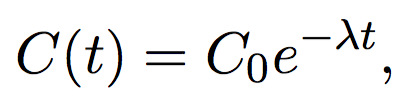
where C0>0 is the initial concentration of iohexol (gm/mL), and λ>0 is the rate of concentration decrease ((gm/mL)min) at time (t). By dividing λ by the amount of the initial iohexol dose (D), we obtain the clinical estimate of GFR (mL/min), which we now want to estimate statistically from observations of plasma iohexol concentration.
Integration of the function in Equation (1) from zero to infinity shows that the area under the curve is given by:
(2)

where AUC is the area under the curve. Thus, if we can estimate the AUC and the constant C0, we will be able to calculate λ, and in turn the GFR, using Equation (2).
Given a set of concentration-time data, we can estimate AUC and C0 as follows. Taking the natural logarithm of both sides of Equation (1) gives the linear expression
(3)

where β1 will be negative. The β values are estimated by fitting a simple linear regression model (Kutner, Nachtsheim, Neter, & Li, 2005, Section 1.8) to the natural log transformed concentration observations. The estimates of β0 and β1 are denoted by b0 and b1, respectively, and other estimates are denoted with hats. Notice that b0 is the estimate of ln(C0) and β1 is the estimate of –λ. The GFR from the single compartment model is then estimated by applying Equation (2):

The smallest number of observations necessary to estimate the GFR using the single compartment model is two, because two points are needed to determine a straight line. Such estimates have zero standard error due to fact that b0 and b1 are uniquely defined by the two observations. However, when more than two observed points are used, the GFR estimate will have non-zero standard error of the GFR, which we will approximate using the delta method. This entails approximating the non-linear function of the two variables b0 and b1 with its first order Taylor series (Stewart, 2012, Section 11.10) about (b0, b1):

so that:

The final variance formula includes population parameters b0 and b1that are unknown, so in practice we replace them with their estimates. In summary:
(4)

where ln(c)=b0 + b1t is the simple linear regression model fit, and
(5)

Here Var(b1), Cov(b0, b1t), and Var(b0) are the components of the variance-covariance matrix (Kutner et al., 2005, Section 5.13) from the simple linear regression model, Equation (3).
Non-Compartmental Model
The assumption of the single compartment model, that the iohexol mixes into the body fluids instantly and uniformly, is an oversimplification. Actually, we can think of the body as having two distinct compartments of fluid, that in the plasma and that in the interstitial fluid. The injected iohexol initially disperses into the plasma quickly, but also begins moving into the interstitial fluid by diffusion once its concentration in the plasma is high enough. This is happening at the same time as a well-functioning kidney is removing the iohexol by filtration. Thus the initial decline in iohexol concentration is actually the sum of two physiological processes – filtration and diffusion. Over time, the concentration of iohexol in the plasma will become lower than that in the interstitial fluid and so diffusion will begin to operate in the other direction, releasing iohexol back into the plasma. The non-compartmental model attempts to be flexible enough to model this complex process without undue mathematical intricacy.
In the case where multiple observations of concentration over time are available, the area under the observed part of the curve can be calculated by the trapezoidal rule (Stewart, 2012, Section 7.7):

where AUCobs is the area under the curve during the observational period. This eliminates the need to make an assumption of the form of the concentration curve. To estimate the area between t = 0 and the first observed point (t1, c1) the single compartment model is used. The line fit through the natural log transform of the first two observed points, (t1, c1) and (t2 , c2), is extrapolated back to t = 0. Integration is then used to find the area from (t0, a0) to (t1, c1), yielding:
(6)

where AUCpre is the area under the curve prior to when observations began and a0 is the estimated y-intercept, a0 = ln(c1)-t1 (ln(C2)-ln(C1)/(t2-t1). A similar approach is used to find the area under the curve from the last observed point (cn, tn) out to infinity. By fitting a simple linear regression model to the last three or more log transformed points, and integrating from the last observed point tn to infinity, the result is:
(7)

where AUCtail is the area under the curve after observations were stopped.
Due to the fact that this approach requires at least three observed points, it is essential to decide how many points to use in the estimation of the decay rate in the tail portion. The model that results in the highest R2 is used, following the approach used by WinNonlin (Pharmasight Corp., 2012) (R2 is a number between 0 and 1 indicating the closeness of a fitted line to observed points, in which 1 indicates perfect fit). The total AUC is the sum of the AUCpre, AUCobs and AUCtail. The estimated GFR is then the dose D divided by the AUC:
(8)

and ln(c)=b0+b1t is least squares fit to the tail with the greatest R2.
The standard error of the estimated GFR was determined by the delta method. We begin with the first order Taylor series of the inverse of AUC about β1:

where A= AUCpre + AUCobs. Then the variance is calculated as follows:

Thus the standard error of the GFR estimated by the non-compartmental method is
(9)

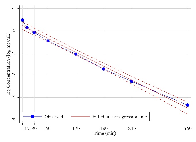
Figure 1. Observed iohexol log-concentration versus time curve for Dog 18, together with estimated simple linear regression line (solid) and 95% CI (dashed). Using the single compartment model, the estimated AUC=126 (Equation (2)), estimated GFRS=2.15 (Equation (4)), standard error of GFRS=0.11 (Equation (5)), and the 95% CI is (0.51, 0.75) (Equation (10)).

Figure 2. Observed iohexol log-concentration versus time curve for Dog 1, together with estimated simple linear regression line (solid) and 95% CI (dashed). The intercept of the fitted line is 0.39, slope=-0.003, and the R2 for the model was 93.3%. Using the single compartment model, the estimated AUC=425 (Equation (2)), estimated GFRS=0.63 (Equation (4)), standard error of GFRS=0.05 (Equation (5)), and the 95% CI is (0.51, 0.75) (Equation (10)).

Figure 3. Observed iohexol concentration versus time curve for Dog 18. Using the non-compartmental compartment model, AUCpre=8.84 (Equation (6)), AUCobs=115 (Equation (5)), the slope of the regression line of tail=-0.009, the R2 for the model is 100%, from a single compartment model of the tail AUCpost=3.93 (Equation (7)), the total AUC=127, estimated GFRN=2.140 (Equation (8)), the standard error of GFRN=0.0008 (Equation (9)), and the 95% CI is (2.13, 2.15) (Equation (10)).

Table 1. Estimated GFR using the single compartment method (GFRS Equation (4), SE(GFRS) Equation (5) and 95% CI Equation (10)).
Standardization for Size
Estimated GFR values are measured in mL/min for each dog. Since there is variation in the body sizes of each dog, the GFR estimates are divided by body weight. This results in estimated GFR measured in mL/min/kg.

Table 2. Estimated GFR using the non-compartmental method (GFRS Equation (8), SE(GFRS) Equation (9) and 95% CI Equation (10)).
Confidence Interval for Estimated GFR
Using the standard errors of the estimated GFR derived above, the 95% confidence interval (CI) for estimated GFR was calculated by the usual method:
(10)

where α = 0.05, n is the number of observations used in the regression model, and t is the student’s t-distribution (Casella & Berger, 2002, Section 5.3.2). For the single compartment model, n is the number of observations, and in the non-compartmental model, n is the number of observations used in the regression model of the tail that gives the highest R2. All data manipulation and analysis were carried out using Stata MP (Version 13.1; StataCorp LP, 2012).
Data Collection
The study was conducted on 21 dogs from a single colony that was maintained at Texas A&M University. These dogs were female carriers of one defective copy of a gene that causes kidney disease (that is, X-linked hereditary nephropathy (XLHN). These female dogs have slowly progressing kidney disease. The iohexol plasma concentration measurement protocol went as follows: dogs were given a bolus intravenous infusion of a mixture of 270mg I/kg of iohexol over 5min into a cephalic vein, then flushed with 2mL of saline. Blood was then drawn at 5, 15, 30, 60, 120, 180, 240, and 360min following Minute 2 of the infusion. This paper is a secondary analysis of data collected for a previous analysis (Nabity et al., 2013). The study protocols were reviewed and approved by the Texas A&M University Institutional Animal Care and Use Committee.
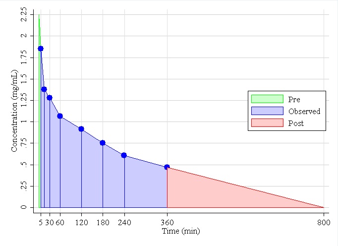
Figure 4. Observed iohexol concentration versus time curve for Dog 1. Using the non-compartmental compartment model, AUCpre=10.01 (Equation (6)), AUCobs=286 (Equation (5)), the slope of the regression line of tail=-0.003, the R2 for the model was 99.1%, from a single compartment model of the tail AUCpost=167.97 (Equation (7)), the total AUC=464, estimated GFRN=0.580 (Equation (8)), the standard error of GFRN=0.0113 (Equation (9)), and the 95% CI is (0.54, 0.62) (Equation (10)).
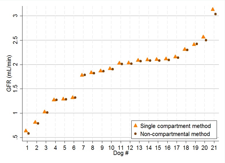
Figure 5. Estimated GFR by single and non-compartmental methods for all dogs, together with 95% CIs. (GFRSEquation (4) and GFRN Equation (8))
RESULTS
The 21 dogs were all moderately large, weighing between 18.0 and 30.3kg with a mean of 22.9kg. Figures 1 and 2 display examples of log-concentration verses time curves used in the single compartment model for two different dogs. In Figure 1 (Dog 18), the linear model appears to fit to the data well except for the initial part of the curve. On the other hand, in Figure 2 (Dog 1) the linear model does not appear to fit as well, and the steepness in the initial part of the curve is more evident. Seeing this curvature in the initial part of the log-concentration versus time curve makes sense anatomically, because this is when the biological marker, iohexol, is being distributed in the body. The distribution phase is followed by the elimination phase, when the kidney is filtering out the marker, which is why the initial curve is followed by a constant decrease. These features impact the R2 of the models, which were 99% to 93%, respectively.
Table 1 lists the means and 95% CI of estimated GFRs for the single compartment method, for all dogs. The table indicates that the standard error, and thus the width of the CI, increases as GFR increases. This is because GFR is a factor in the standard error (Equation (5)).
Figures 3 and 4 show examples of concentration verses time curves using the non-compartmental model for the same two dogs. Both figures are on a same scale. However, notice that in Figure 4 the concentration at 360min is still high compared to that in Figure 3, where the concentration is almost at zero. Thus, the AUCtail is considerably larger for Dog 1 than Dog 18. Table 2 lists the means and 95% CI of estimated GFRs for the non-compartment method of all dogs. Notice the R2 values in both tables are very high, all greater than 99%. This time, the standard error (and thus the width of the CI) decreases as GFR increases. This is due to the term cn/b1 in Equation (9), which decreases so rapidly as GFR increases that even though it is divided by AUC, the standard error is still decreasing, particularly when the GFR is small.
Figure 5 displays the GFRs estimated by both methods for all dogs together with their 95% CI. Notice that CIs from the non-compartmental method are much narrower than that for the single compartment method, but the two estimated values from the two methods are quite similar. Thus, when eight points between 5 and 360minutes are used, the single compartment model provides an adequate estimate of the GFR, despite having a comparatively wide CI.
DISCUSSION AND CONCLUSIONS
GFR is used for evaluating renal function and is estimated using the relationship between the serial plasma concentrations of an exogenous marker and time. This paper demonstrates how the delta method can be applied to approximate the standard error of estimated GFR, thus allowing the provision of an interval estimate for GFR, using two models: the single compartment and the non-compartmental. These results were applied to data on 21 dogs, consisting of eight observations between 5 and 360min. As a result, we have found that the non-compartmental model results in very narrow CIs, and that the GFR estimate from single compartment model is close to that of the non-compartmental model, despite the fact that its CI is considerably wider.
The CI for the single compartmental model is wide because it fits a simple linear regression model to all the log-concentrations and, because the iohexol dissipates quickly into the interstitial fluid initially, the log-concentration curve is not a straight line. On the other hand, the non-compartmental model uses the observed concentrations in a deterministic way, meaning that only the area from the unobserved tail portion of the concentration curve is estimated statistically. While this appears to be beneficial for obtaining small standard errors, it actually gives little information as to the accuracy of the point estimate. However, the close relationship between the GFR estimates from the two methods, at least in this case of eight observed points for each dog, allays that concern to some extent.
There is no previous literature for estimating standard errors of GFR estimated in a direct manner. Complex treatments of interval estimation in pharmacokinetic–pharmacodynamic modeling, while valuable for their rigor, are largely impenetrable to practitioners and clinicians (Bauer, Guzy, & Ng, 2007; Csajka & Verotta, 2006). Thus this paper constitutes a valuable and accessible contribution to the literature on interval estimation for estimated GFR.
REFERENCES
Bauer, R. J., Guzy, S., & Ng, C. (2007). A survey of population analysis methods and software for complex pharmacokinetic and pharmacodynamic models with examples. The AAPS Journal, 9(1), E60-E83.
Bagshaw, S. M., & Bellomo, R. (2009). Kidney Function Tests and Urinalysis in Acute Renal Failure in Ronco, C., Bellomo, R., & Kellum, J., (Eds.) Critical Care Nephrology (2nd ed.) (pp. 253). Philadelphia, PA. Saunders Elsevier.
Casella, G., & Berger, R. L. (2002). Statistical inference (Vol. 2)(Section 5.5.4): Pacific Grove, CA: Duxbury.
Csajka, C., & Verotta, D. (2006). Pharmacokinetic–pharmacodynamic modelling: History and perspectives. Journal of Pharmacokinetics and Pharmacodynamics, 33(3), 227-279.
Dorfman, R. (1938) A note on the d-Method for Finding Variance Formulae. The Biometric Bulletin, 1(4), 129-137.
Heiene, R., & Moe, L. (1998). Pharmacokinetic aspects of measurement of glomerular filtration rate in the dog: a review. Journal of Veterinary Internal Medicine, 12(6), 401-414.
Kutner, M. H., Nachtsheim, C. J., Neter, J., & Li, W. (2005). Applied Linear Statistical Models. Chicago, IL: McGraw-Hill Irwin.
Nabity, M. B., Lees, G. E., Boggess, M., Yerramilli, M., Obare, E., Yerramilli, M., Aguiar, J., Relford, R. (2013). Week-to-week variability of iohexol clearance, serum creatinine, and symmetric dimethylarginine in dogs with stable chronic renal disease. Journal of Veterinary Internal Medicine, 27(3), 734-734.
Paine, S. W., Ménochet, K., Denton, R., McGinnity, D. F., & Riley, R. J. (2011). Prediction of human renal clearance from preclinical species for a diverse set of drugs that exhibit both active secretion and net reabsorption. Drug Metabolism and Disposition, 39(6), 1008-1013.
WinNonlin [Computer Software]. (2012). Princeton, NJ: Pharsight Corp.
StataCorp LP [Computer Software]. (2012). 4905 Lakeway Drive, College Station, TX: StataCorp LP.
Stevens, L. A., Coresh, J., Greene, T., & Levey, A. S. (2006). Assessing Kidney Function — Measured and Estimated Glomerular Filtration Rate. The New England Journal of Medicine, 354(23), 2473-2483.
Stewart, J. (2012). Calculus Early Transcendentals (7 ed.) (Section 11:10). Belmont CA: Cengage.
Tanner, G. (2009). Kidney Function. In R. Rhoades & D. Bell (Eds.), Medical Physiology: Principles for Clinical Medicine (pp. 396-397). Philadelphia, PA: Lippincott Williams & Wilkins.
Ver Hoef, J. M. (2012). Who invented the delta method? The American Statistician, 66(2), 124-127.