

Author: Benjamin Ripman
Institution: Bowdoin College
Date: November 2007
ABSTRACT
Using interferometric maps, the statistical properties of the velocity fields traced by H2O masers in five galactic regions of star formation were investigated. In a previous work, Strelnitski et al. (2002) concluded that H2O masing spots in such regions appear to probe highly intermittent supersonic turbulence and demonstrated that the two-point velocity correlation functions for the line-of-sight components of velocity traced by the masers could be approximated by power laws, with the exponents near the classical Kolmogorov value of 1/3 expected for high-Reynolds number incompressible turbulence. In the present project, we undertook a more in-depth investigation of the two-point velocity correlation functions for the previously studied H2O sources and for one new source with published interferometric maps. We confirm that the velocity correlation functions can be satisfactorily approximated by power laws for all of these sources, but we observe that a single power-law fit for the whole observed span of spatial scales is inadequate to describe the data applied over constrained ranges of scale. At intermediate scales, we found that the power law exponents were near the Kolmogorov value. At smaller scales, however, there was a pronounced increase of the slopes, which may be regarded as an indication that appreciable dissipation of energy in supersonic turbulence begins at spatial scales considerably larger than both the Kolmogorov microscale and the possible dissipation scale due to the formation of random shock waves, as hypothesized by Strelnitski et al. At the largest scales, we found a pronounced flattening of the slopes, which we attribute to the contamination of the turbulent velocity field at these scales by regular components of motion (expansion and rotation).
INTRODUCTION
The phenomenon of turbulence is one of the least well-understood subjects in the modern theory of fluid mechanics. Although turbulence remains inaccessible to strict analytical investigation, our understanding of incompressible (subsonic) turbulence has improved immensely over the last century (Kundu, 2004). In the mid-20th century, Andrey Kolmogorov developed a phenomenological theory of incompressible turbulence, predicting that kinetic energy in turbulent flows should cascade down from the characteristic injection scale through an "inertial subrange" in which no significant energy loss occurs, finally dissipating on a "microscale" at which viscous effects become dominant (Kolmogorov, 1941a, 1941b, 1941c). Laboratory experiments, observations, and numerical simulations have since confirmed the general validity of these results (Frisch, 1995).
Unfortunately, experimental and analytical exploration of highly supersonic (compressible) turbulence poses much greater challenges. Production of high-Mach number turbulence in the laboratory is exceedingly difficult. Computer simulations of supersonic turbulence may shed some light on this subject, but with the computing power available today, these simulations lack the dynamical range required to follow the turbulent cascade over the multiple decades in spatial scale that may separate the energy injection scale and the various hypothesized dissipation scales. Moreover, computer simulations of high Mach number, driven supersonic turbulence are usually carried out in the isothermal regime. This may be an unphysical approximation, as it would require rapid injection of heat energy into those regions of the supersonic flow that undergo rarefaction. Adiabatic simulations have mainly focused on transonic, decaying turbulence.
Fortunately, nature seems to have provided us with an opportunity to directly explore the properties of highly supersonic turbulence. The interstellar medium (ISM) is characterized by huge distances, high velocities, and low densities. These factors combine to produce very high Reynolds numbers, and as a consequence, the ISM is very unstable against turbulization. Various groups have suggested that the gas clouds in star forming regions are turbulized by the outflow of matter and energy from newly formed stars. Given the observed dispersion of velocity within these regions often as high as 500 km s-1 and the speed of sound in the interstellar medium (ISM) typically on the order of 1 km s-1 - these turbulent flows are undoubtedly supersonic. In fact, these flows possess Mach numbers in the tens or hundreds.
Some of these regions are studded with natural masers - bright, compact sources of microwave radiation, with the average masing "hot spot" size on the order of 1 AU (Gwinn, 1994). The typical extent of the regions containing these masers is approximately 105 AU (e.g. Strelnitski et al., 2002). The masers can therefore be treated as point-like probes of the velocity field of the turbulent medium in which they are embedded, allowing us to study the detailed statistical properties of this medium. Walker (1984), Gwinn (1994), and Strelnitski et al. (2002) undertook such analysis, demonstrating that the two-point velocity increments in several galactic regions of star formation display power-law dependence on maser separation. Strelnitski et al. (2002) also demonstrated that the spatial distribution of the maser spots is fractal, with a corresponding fractal dimension d ≤ 1.
In the cited papers, most of the sources were treated globally, in the sense that all of the linear scales involved were considered together. However, the point distribution on the graphs that were used to find the two-point velocity correlation functions often showed obvious deviations from a linear fitting. This paper presents the results of a more detailed study of the statistics of the velocity fields traced by H2O masers in regions of star formation. We also revise the determination of the fractal dimension of the H2O maser clusters. In Section 2, we discuss the methods by which we examined these properties. We present the results of our analysis for five H2O maser sources in Section 3, and we discuss the implications of those results for the theory of supersonic turbulence in Section 4. Our conclusions are summarized in Section 5.
METHOD OF ANALYSIS
We investigated the two-point velocity correlation functions for the line-of-sight component of velocity traced by the H2O masers in five galactic regions of star formation: W49(North), W51(Main), W51(North), SgrB2(Main), and SgrB2(North). In performing this analysis, we assumed that any power-law scaling relationship that exists for velocity vectors in three-dimensional space holds (with the same exponent) for the dependence of the line-of-sight component of velocity on projected distances. This assumption holds true if the velocity field in question is isotropic. We also assumed that the spherical celestial coordinates of the maser features could be well-approximated by rectangular Cartesian coordinates. This is an excellent approximation, given that every region studied was less than 10 arc seconds across.
The two-point velocity correlation function is defined as follows:

Equation 1 1313
In equation (1), the vector r determines the projected position of one point in the plane of the sky and the vector l defines the offset with projected length l to another point. The scalar quantity v represents the line-of-sight velocity at each point.
Our procedure is as follows: the range of maser spot separations, which typically span approximately 4 orders of magnitude, is divided into bins, with a constant logarithmic distance S between the centers of the bins. Using the VLBI relative position data, the procedure finds all of the maser pairs that fall within each separation bin and calculates their average velocity difference. The mean velocity differences within each bin are then plotted as a function of separation on two log-log graphs.
On the first graph, a least-squares linear fit is applied to the entire dataset and used to find the power law exponent q and its associated uncertainty. On the second graph, linear fits are applied to three limited, but overlapping, ranges in separation. A least-squares quadratic fit is also applied to the entire dataset on the first graph; this allows for a quick visual assessment of the relative qualities of the overall best-fit line and the best-fit lines applied over limited separation ranges.
We also calculated the fractal dimension of each source using the "density-radius" method (e.g. Strelnitski et al., 2002). This method is based on the formula for the relationship between mass and radius for objects of integer dimension d, so that M~rd
This equation may be used to define any object's dimension, including those objects whose average density changes in a self-similar way with spatial scale (Mandelbrot, 1982). These objects are said to be fractal, and their dimension d is non-integer. Average density ρ within a volume V is M/V. Therefore,

Equation 3
Where d' is the dimension of the supporting space, e.g., d' = 2 for a plane. If the dimension of the object equals the dimension of the support, ρ is a constant. If not, ρ is a function of r. The steepness of this function depends on d. Differentiating Equation 3 yields,

Equation 4
or

Equation 5
One can therefore determine the dimension of an object by measuring the slope of log(σ) vs. log(r) and adding the dimension d' of the supporting space to this value. We defined σ as follows when finding the slope of log(σ) vs. log(r):

Equation 6
In equation 6, σ (r) is the average number density of points at a distance r from each maser in the region being studied.
Since the regions being studied are finite in size, edge effects inevitably contaminate the data at large values of r; the calculated number density drops off to zero as r increases, so the calculated fractal dimension is lower than the actual fractal dimension. Our procedure compensates for edge effects by discounting the most contaminated portion of the data those points corresponding to the largest values of r - but it is inevitable that the calculated fractal dimension for each source is a slight underestimate.
RESULTS
Examples of the graphs used for the two-point velocity correlation analysis are presented in figures 1-5, and the final results are summarized in Table 1. Each graph is derived from a dataset corresponding to one particular interferometric observation. Some sources were mapped multiple times, over separate epochs, with different facilities. Moreover, the coordinates of the maser spots observed during different epochs were given with respect to different reference features. Therefore, it is impossible to present a single graph for each source that integrates all of the information available on that source.
3.1. W49(North)
In our analysis of the W49(North) region, we used VLBI and VLA data reported in three different papers (Gwinn, 1992, 1994; McGrath, 2004). W49(North) is composed of several compact HII regions in a rotating ring formation approximately 1 pc in diameter. The turbulent eddies that form within this region may be driven by the ring's large-scale rotation (Gwinn, 1992).
W51(Main)
We used VLBI data reported in two papers in our analysis of the W51(Main) region (Genzel, 1981; Imai, 2002). The transverse motions of the sources in W51(Main) appear chaotic; the pumping of masers within this region has been attributed to the interaction between stellar winds and density inhomogeneities in the surrounding clouds (Genzel, 1981).

Fig. 1 Two-point velocity correlation function for H2O masers in W49(North), plotted with a logarithmic bin size of 0.25. (a) Least-squares linear and second-order polynomial fits applied to the entire dataset. (b) Linear fits applied to three separation ranges (low, medium, and high-separation). Observational data from Gwinn (1994).

Fig. 2 Same as Fig. 1, for H2O masers in W51(Main). Data from Genzel (1981).
W51(North)
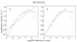
Fig. 3 Same as Fig. 1, for H2O masers in W51(North). Data from Imai (2002).
We used VLBI data reported in two papers in our analysis of the W51(North) region (Schneps, 1981; Imai, 2002). This region contains an expanding flow with a regular velocity of ~70 km s-1. However, substantial residual motions are also observed in this region (the observed masers have a velocity dispersion of ~100 km s-1), which may indicate that the flow itself is turbulent (Imai, 2002).
[b/SgrB2(Main)
We used VLA data reported in McGrath (2004) in our analysis of the SgrB2(Main) region.

Fig. 4 Same as Fig. 1, for H2O masers in SgrB2(Main). Data from McGrath (2004).
SgrB2(North)
We used VLA data reported in McGrath (2004) in our analysis of the SgrB2(North) region.

Fig. 5 Same as Fig. 1, for H2O masers in SgrB2(North). Data from McGrath (2004).
Overall Results
The power law exponents derived from the least-squares linear fits to various separation ranges for each of the regions studied are presented in Table 1. This table also presents the fractal dimension calculated for each region.
DISCUSSION
The average RMS deviation of the plotted points from the least-squares linear fits applied to the entire data sets (0.20) was notably larger than for the quadratic fit (0.14). This indicates that the slope of the power-law fit changes with maser pair separation, which justifies the use of the constrained fits. As seen in Table 1, the average power law exponent q is compatible with the Kolmogorov value of 1/3 for the entire range of separations and for the intermediate separation ranges. However, q is noticeably higher than the Kolmogorov value for the smallest separation ranges and considerably lower than the Kolmogorov value for the highest separation ranges.

Table 1 Best-fit slopes for various ranges of maser pair separation and calculated fractal dimension for each region.
Before discussing the implications of these results, it is important to note the following. Kolmogorov's predictions were put forward in the context of incompressible turbulence and rest on the assumption that the specific energy transfer rate, ρv3/l, is constant along the scales. Since the specific density ρ remains constant in an incompressible fluid, the above assumption reduces to v3/l = const, or v ~ l1/3. However, the density distribution in a supersonically turbulent medium is, by definition, inhomogeneous. Fleck (1996) showed that for a simple case where one can describe the compressibility of the fluid on all scales with a single parameter α , the above scaling law is modified to v ~ l1/3 + α. Very little is known about the possible values of α in real fluids and about possible dependence of these values on the scale. One cannot exclude that at larger scales α is very small, and that it becomes significant only around the dissipation scale. In this case, supersonic turbulence will not differ, phenomenologically, from incompressible turbulence it will possess an "inertial subrange," with a velocity spectrum close to Kolmogorov.
The observed steepening of the power law fits over the smallest separation ranges most probably indicates that energy dissipation in supersonic turbulent flows probed by H2O masers begins at scales larger than both the Kolmogorov microscale and the dissipation scale hypothesized by Strelnitski et al. (2002).
The flattening of the slope at larger separations most probably reflects the fact that the relative regular motion of the maser features is the dominant factor at the greatest spatial separations. As the separation between masers increases, that regular motion will increasingly contaminate the statistics of the turbulent motion; the average difference in velocities at these scales will relax to some relatively constant velocity dispersion that characterizes the region as a whole. Interestingly, the average power-law exponent for the highest separations, 0.08 ± 0.10, is similar to that predicted by Strelnitski et al. for the case of masers randomly distributed across a uniformly expanding, spherical gas shell.
Our results confirm Strelnitski et al.'s conclusion that H2O maser clusters have fractal dimensions ≤ 1. As discussed in Strelnitski et al., the fractal distribution of the maser spots, which are most likely embedded in regions of turbulent energy dissipation, is an indication that turbulence is intermittent, and the low fractal dimensions calculated indicate that the degree of intermittency is high, implying that the filling factor of active turbulence is low.
CONCLUSIONS
A detailed investigation of the velocity and spatial distribution statistics of H2O masers in regions of star formation reveals the following:
1) For most of the sources, the power index of the two-point velocity correlation function for the whole span of scales occupied by maser spots is compatible with its classical (Kolmogorov) value for high-Reynolds number incompressible turbulence.
(2) However, the slope of the log-log dependence of velocity increments on point separations characteristically changes with the scale in most of the investigated sources, decreasing from the smallest to the largest scales. The steeper-than-Kolmogorov slope at smaller scales can be explained by an energy dissipation rate that increases with decreasing scale, whereas the shallower slope at the highest scales is probably due to contamination of the turbulent pulsations by components of regular velocity (expansion and/or rotation).
(3) Analysis of the two-point velocity correlation functions for these regions seems to support the notion that supersonic turbulence has an inertial subrange of scales where energy dissipation is insignificant. However, appreciable energy dissipation appears to begin at scales larger than both the Kolomogorov microscale that arises from viscous effects and the microscale arising from massive production of random shocks postulated by Strelnitski et al.
(4) All the regions analyzed were found to have fractal dimensions less than or on the order of unity, which indicates a high degree of intermittency in the probed supersonic turbulence.
The author would like to thank Dr. V. Strelnitski for his guidance and support. This project was supported by the NSF (Research Experience for Undergraduates) and the Nantucket Maria Mitchell Association.
REFERENCES
Fleck, R.C., Jr. (1996) Scaling Relations for the Turbulent, Non,Self-gravitating, Neutral Component of the Interstellar Medium. The Astrophysical Journal 458, 739-741.
Frisch, U. (1995) Turbulence. Cambridge: Cambridge University Press.
Genzel R et al. (1981) Proper motions and distances of H2O maser sources. II - W51 MAIN. The Astrophysical Journal 247, 1039-1051.
Gwinn, C. R. (1994) Physical structure of H2O masers in W49N. The Astrophysical Journal 429, 253-267.
Gwinn, C.R. et al. (1992) Distance and kinematics of the W49N H2O maser outflow. The Astrophysical Journal 393, 149-164.
Imai, H. et al. (2002) 3-D Kinematics of Water Masers in the W 51A Region. Publications of the Astronomical Society of Japan 54, 741-755.
Kolmogorov, A.N. (1941a) The local structure of turbulence in incompressible viscous fluid for very large Reynolds numbers. Doklady Akademii Nauk SSSR 30, 301-305.
Kolmogorov, A.N. (1941b) On the logarithmically normal law of distribution of the size of particles under pulverisation,. Doklady Akademii Nauk SSSR 31, 99-101.
Kolmogorov, A. N. (1941c) On degeneration of isotropic turbulence in an incompresible fluid. Doklady Akademii Nauk SSSR 31, 538-540.
Kundu, P. & I. Cohen (2004) Fluid Mechanics. London: Elsevier.
Mandelbrot, B. B. (1982) The Fractal Geometry of Nature. New York: Freeman.
McGrath, E. J. et al. (2004) H2O Masers in W49 North and Sagittarius B2. The Astrophysical Journal Supplement Series 155, 577-593.
Schneps, M. H. et al. (1981) Proper motions and distances of H2O maser sources. III - W51NORTH. The Astrophysical Journal 249, 124-133.
Strelnitski, V. et al. (2002). H2O Masers and Supersonic Turbulence. The Astrophysical Journal 581, 1180-1193.
Walker, R.C. (1984) H2O in W49N. II - Statistical studies of hyperfine structure, clustering, and velocity distributions. The Astrophysical Journal 280, 618-628.