

Authors: Ryan Hayes, Michael Freed
Institution: Baylor University
Date: March 2007
Abstract
Dust particles in a protoplanetary disk coagulate into larger bodies which eventually form planetesimals. When the dust particles stick together, they form fluffy aggregates which often have a self similar structure characterized by the fractal dimension. The fractal aggregates can couple more closely to the gas in the nebula, which decreases their relative velocities. Since some of the gas particles are ionized, the dust becomes charged due to collisions with free ions and electrons. These dust properties, relative velocity and charge, have a large effect on both the coagulation rate and the fractal dimension. A fifth order Runge-Kutta algorithm was used to model the coagulation of dust particles for various charge and size distributions. The electrostatic forces between aggregates were calculated using the monopole and dipole terms of the potential of the charged grains. The fractal dimensions of the aggregates were calculated using the spherically averaged density (SAD) and the Hausdorff dimension. Comparisons between the two results are presented. Two charge redistribution algorithms were used to investigate the distribution of electric charge on the fractal aggregates. One algorithm assumed conservation of charge during collisions, and a dipole moment was calculated from the physical geometry of the grain. The other found the equilibrium charge distribution from an orbital motion limited (OML) line of sight approximation. In general the OML approximation predicted substantially lower charges on the aggregates which would improve the coagulation rate.
Introduction
It is widely believed that planets form from the gas and dust in a protoplanetary disk surrounding a newly formed star. Objects larger than 1 km can decouple from the gas and begin to coagulate through gravitational interactions. However, on smaller size scales, effects from the gas in the disk, such as gas drag and dust charging, also play a major role. Until recently, processes that govern the dynamics on this scale were poorly understood (Weidenschilling and Cuzzi 1993), but recent numerical models of dust coagulation have led to an increased understanding of these processes (Matthews and Hyde 2004; Richardson 1995; Ossenkopf 1993).
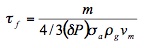
In a protoplanetary disk, there are several sources of relative velocities between particles including Brownian motion, sedimentation, radial drift, and gas turbulence (Weidenschilling and Cuzzi 1993; Wurm and Blum 1998), all of which depend on the properties of the gas. Sedimentation, radial drift, and gas turbulence also depend on τƒ , the gas-grain stopping time, which is given by
article_933_order_10
(Equation 1)
where m is the mass of the particle, σa is its cross sectional area, δP is the momentum transfer efficiency factor of about 1.11±0.17, ρg is the density of the gas, and νm is the mean thermal velocity of the gas (Wurm and Blum 1998). Smaller particles have a very short stopping time, which means they are well coupled to the gas, and respond almost instantly to changes in gas velocity. The gas-grain stopping time depends on both the properties of the gas through ρg and νm, and on the physical properties of the aggregate through m and σa. The ratio of m and σa can be determined from the fractal dimension. Since the fractal dimension affects the stopping time, it also affects the relative velocities of small particles.
If the relative velocities between grains are too low, the coagulation rates will also be low. If the relative velocities are too high, the particles can crush, fragment, or bounce rather than sticking together. Dust particles that collide with sufficiently low velocities (~1 m/s) will stick due to Van der Waals forces (Chokshi, Tielens, and Hollenbach 1993; Haghighipour 2005). Van der Waals forces are contact forces. The surface of a material is less stable than the interior, so when particles touch their surfaces assume a lower energy state, and a force is required to break contact. Although relative velocities between dust grains may exceed the sticking velocity, a sticking probability of unity is usually assumed in numerical simulations. The validity of this assumption is discussed by Blum and Wurm (2000).
Because the particles stick at their first point of contact, the aggregates have an open structure. The center of the aggregate tends to be more dense, while the outer portions are less dense with a few protruding arms. The fractal dimension is a measure of the openness of the structure. While Euclidean objects such as a line, a plane, or a cube have integral dimensions of one, two and three, respectively; a fractal object can have a non-integer dimension. The fractal dimension is only strictly defined for objects extending to infinite or infinitesimal size scales, but it can take on an approximate value in finite objects between two size scales. The bounding size scales are the limits at which self similarity breaks down, or in the case of dust aggregates, when sub-clusters of the aggregate cease to look like the cluster they are members of. Thus the size limits range from the aggregate size to the size of a single dust grain. The mass of a fractal aggregate is given by
m∝agDf (Equation 2)
where ag is the radius of gyration, and Df is the fractal dimension (Blum and Wurm 2000). Common calculations of the fractal dimension of dust aggregates in a protoplanetary disk yield Df ≈1.9, however, this value is sensitive to initial conditions.
The gas in a protoplanetary disk may be partly ionized due to UV rays. This creates a plasma environment which leads to an accumulation of charge on the dust particles (Horányi 1996; Bringol and Hyde 1997). The charge on a grain has a large effect on coagulation rates. It can cause the collisional cross section to increase or decrease due to electrostatic repulsion or attraction (Ossenkopf 1993), or even prevent coagulation if the relative velocities are not great enough to overcome the coulomb barrier (Matthews and Hyde 2004). Thus the charge on each dust particle or aggregate is critically important in determining collision outcomes and coagulation rates.
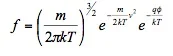
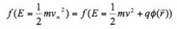
Grain charging occurs because of unbalanced currents to the grain in the form of primary ion and electron flux, and secondary electron emission (Horányi 1996). Orbital Motion Limited (OML) theory is used to approximate the charge on a spherical dust particle due to the primary currents (Laframboise and Parker 1973). It requires that there be no collisions between ions, which is a valid approximation if the mean free path of the ions is much larger than the effective potential well of the charged grain. Under this restriction, a kinetic energy distribution at infinity will gain energy in the potential well, but maintain its shape. Thus, for a distribution function f,

article_933_order_15
(Equation 3)
where v∞ is the velocity at r = ∞, and φ(r) and v are the voltage and speed of the ions at any point r (Laframboise and Parker 1973). If all positive energy orbits connect back to infinity, then the energy distribution is isotropic throughout velocity space, which means independent of direction. In order to find the charging current, one must calculate the flux through the surface bounding the dust particle. Orbits which have already passed through a surface once must not be counted again. It is impractical to find which orbits have passed through a surface in situations without a high degree of symmetry. As a result, OML theory is of limited use in situations without spherical, elliptical, or cylindrical symmetry. For a spherical dust grain, assuming equal electron and ion temperatures in a hydrogen plasma, the equilibrium voltage and charges are given by the well known formulas
article_933_order_16
(Equation 4)
q=4πε0aφ (Equation 5)
where k is the Boltzmann constant, T is the temperature of the plasma, and a is the radius of the grain (Spitzer 1978). Secondary electron charging occurs when energetic electrons strike a dust grain and knock off other electrons. Secondary electron yield can have a large effect on equilibrium grain charge in plasmas with temperatures above 5 eV, even leading to oppositely charged grains (Horanyi and Goertz 1990). It is neglected for simplicity in the present work. A complete description of the phenomenon is given by Bringol and Hyde (1997) and Chow, Mendis, and Rosenberg (1993).
Methods
The Aggregates
A dust aggregate builder was implemented using MATLAB, as described in (Matthews, Hayes, Freed, and Hyde 2006). Aggregates were built with dust particles from a flat size distribution with the radius a between 1 μm and 6 μm. Three different dust populations were given like, neutral, and opposite charges. The like charged particles were charged to a potential of -1 V, corresponding to a plasma temperature of 4600 K, with charges calculated by (Equation 5). This reflects charging from primary currents alone. In the oppositely charged population, particles with a < 4 µm had a charge of -1 V, and particles with a ≥ 4 µm had a charge of +4 V. This reflects the conditions in (Horanyi and Goertz 1990), which included optimistic secondary electron emission.
In each model, three generations of aggregates were built. The first generation was built by shooting single particles at a seed particle until the resultant aggregate contained twenty spherical monomers. After each addition, the aggregate characteristics were saved in a library. In the second generation, aggregates stored in the first generation were used for the seed aggregate as well as the incoming aggregates, so that the colliding aggregates contained between two and twenty monomers. This continued until there were 200 monomers in the target aggregate. In the third generation, a mixture of aggregates from the first and second generation was fired at the seed. 75% were chosen from the second generation, and 25% were chosen from the first generation. Collisions occurred until the target aggregate contained 2000 monomers.
Calculation of Fractal Dimension
The fractal dimension was first defined by Mandelbrot (1983). Since it is only strictly defined for objects extending to infinity, the smaller the aggregate, the more approximate the value of Df, the fractal dimension. One method used to approximate a fractal dimension is the spherically averaged density (SAD) (Richardson 1995). For a monodisperse population, where all of the dust grains are the same size, the spherically averaged density ρ is related to the number of particles N by
ρ∝Nγ (Equation 6)
where γ is a constant related to the fractal dimension by
article_933_order_17
(Equation 7)
For populations with a size distribution, the mass of the aggregate must be used in place of the number of monomers. Because the mass, volume, and density are related to the size of the aggregate by
m∝rDf (Equation 8)
V∝r3 (Equation 9)
ρ∝rDf-3 (Equation 10)
where r is any characteristic radius, usually chosen to be the radius of gyration, r can be eliminated from (Equation 8) and (Equation 10), leaving
ρ∝mγ (Equation 11)

article_933_order_17
(Equation 12)
Then γ can be found from the slope of a log-log plot of ρ versus m. The spherically averaged density of a single aggregate is too rough to fit a curve, so the total mass and the radius of maximum extent were used to calculate spherically averaged densities for the population. Finally a curve was fit to the data to find the average fractal dimension for each generation as well as the entire population.
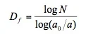
An alternate method of calculating the fractal dimension was also employed. The fractal dimension may be obtained from calculating the Hausdorff dimension, or the capacity dimension (Goldstein, Poole, and Safko 2002). The Hausdorff dimension is calculated by dividing each dimension of a space into segments of length a. If the space is a0 on a side, and N of the subspaces defined by a are filled, the Hausdorff dimension is defined as
article_933_order_18
(Equation 13)
For example, if a cube of length a0 on a side is divided into a0/a pieces on each side, it would contain N = (a0)3 boxes, thus the Hausdorff dimension Df corresponds to the Euclidean dimension of three. To calculate the Hausdorff dimension of a fractal aggregate, a cube centered on the center of mass of the aggregate and oriented along the three principle axes was sized so that it just contained the aggregate. The cube was divided into a0 = 200 points on each side. If a test point was inside a dust grain in the aggregate, its box was added to N, the total number of test points contained within the aggregate structure.
Aggregate Charging
To get an accurate picture of the equilibrium charge distribution on a fractal aggregate, one must model firing individual electrons and ions at the aggregate from all angles, with varying offsets at varying velocities. This is computationally intensive, and completely impractical. Therefore two models of charge redistribution were implemented. The first model relied on charge conservation, and the second was derived from orbital motion limited theory (OML).
The charge conservation method was used in our model because it required less CPU time. After a successful collision, the total charge was assumed to be conserved, but was redistributed across the monomers in the aggregate according to the law
(Equation 14)
where di is the distance from the ith particle to the center of mass (Matthews and Hyde 2004). This heuristic redistribution algorithm reflects a dielectric material. In a dielectric, the charge will tend towards the extremities of the aggregate because this is a lower energy state than having all the charge concentrated at the center. In a conductor, one can move the charges around until the voltage is constant throughout the aggregate.
In order to get a better approximation of the charge distribution on an aggregate, orbital motion limited (OML) theory was used with a line of sight approximation. The primary difficulty in OML is removing all the orbits from velocity space which have already intersected the target once. (Another difficulty is that OML may not apply in a dusty plasma where the potential of the dust grains is described by a Yukawa potential rather than a Coulomb potential (Kennedy and Allen 2003; Laframboise and Parker 1973). After the removal of these orbits, the flux is calculated from the remaining orbits. The current density to any point is given by
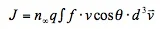
(Equation 15)
where n∞ is the number density outside the potential well, q is the charge on a particular ion species, f is the distribution function, θ is the angle at which an orbit or path intersects the surface, and the integration is carried out over the velocity space d3v of all orbits which intersect the surface for the first time. The distribution outside the potential well was assumed to be Gaussian. Substituting the total energy from (Equation 3) into the Gaussian distribution yields
(Equation 16)
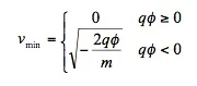
The minimum velocity of this distribution is given by
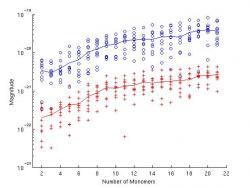
Figure 4. The dipole magnitudes for both charging schemes in Coulomb-meters. The OML is plotted with crosses, and the conservation model is plotted with circles. The mean of both models is also plotted. The mean magnitude follows a roughly linear progression, but is presented on a semi-log plot for clarity between the orders of magnitude.
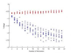
Figure 5. The surface potential given by the two charging methods in Volts. The OML potential is plotted with crosses, and the conservation model voltage is plotted with circles. The voltage is calculated using only the monopole term, and the distance from the monopole is obtained from the radius of maximum extent, i.e. the distance from the center of mass to the far side of the furthest dust grain.
(Equation 17)
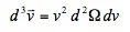
since an approaching particle can have neither negative speed nor a negative total energy. The substitution of
(Equation 18)
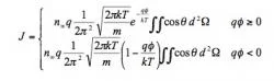
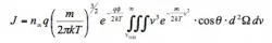
into (Equation 15), where d2Ω is a differential solid angle, along with (Equation 16), results in the expression for the charging current.
(Equation 19)
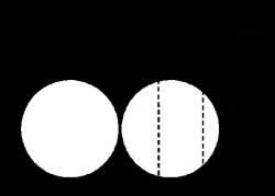
Figure 6. The OML line of sight model would predict that both charging currents would have completely free lines of sight to the right of the center of the right sphere. The real regions where they have unobstructed currents are shown to be right of the dotted lines. The unobstructed region for the ions is smaller than the unobstructed region for the electrons.
where d2Ω is integrated over the solid angles of the unobstructed orbits. In our model it was assumed that electrons and ions approaching the atom move in a straight "line of sight". The flux to a point on the surface of a grain coming from a direction obstructed by any dust grain, including itself, is excluded from the integration as an orbit which has already intersected the aggregate. This approximation gets poorer as the aggregate accumulates charge. The integration range is really a function of velocity, since faster particles will have less curvature to their orbits due to interaction with the aggregate's electric field. However, in a line of sight approximation, the deflection of the ions and electrons is assumed to be negligible so that the d2Ω integration will be independent of speed and may be factored out of the dv speed integral. Evaluating (Equation 19) with this assumption yields
(Equation 20)
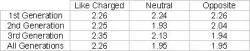
Figure 1. The fractal dimensions given by the spherically averaged density.
where J is the current density for each ion species, θ is the angle between the normal to the surface and the direction to the solid angle Ω, and Ω ranges over all unobstructed paths to a single point on the grain. To find the total current to the grain, one must integrate the current density J for each ion species over the entire surface of the aggregate. In the case of an isolated spherical dust grain, where only orbits coming from inside the grain itself must be ignored, the solid angle integral reduces to a factor of π and the surface integral reduces to a factor of 4πa2. Setting the electron and the ion currents equal to each other yields the expected result (Equation 4).
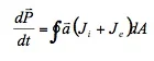
Because current does not flow inside of a dielectric, charges impacting different regions of a dielectric aggregate will remain near the point of impact. Therefore the current to each dust grain in an aggregate was calculated separately. Both monopole and dipole currents were calculated, the dipole current being the time derivative of the dipole moment. The dipole moment approximates the distribution of charge on the grain. These currents are given by
article_933_order_6
(Equation 21)

article_933_order_7
(Equation 22)
where dA is the differential surface area of the sphere, and a is the vector pointing from the center of the sphere to the surface element dA.
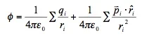
The integrals in (Equation 20, Equation 21, and Equation 22) were calculated numerically. In each time step the potentials at each point on the surface of all the grains were calculated from the charge qi and dipole moment pi on each grain.
article_933_order_8
(Equation 23)
The current densities at each point on the surface of the grain were calculated from the potentials using (Equation 20), and the charge and dipole currents to each grain were calculated from the current densities using (Equation 21 and Equation 22). Finally the charges and dipoles on each grain were updated, and the potential was calculated for the next step. Charging was simulated for 500 time steps, and a visual check of the charging history ensured that the currents had reached equilibrium.
Two hundred sample aggregates, ten of each size, were chosen from the first generation of the like charged population. The OML line of sight charging algorithm was applied with a temperature of 4600 K, because it was determined that this plasma temperature lead to a charge of -1 V, which would allow direct comparison with the charge conservation method. A plasma number density of 5 × 10⁸ m-3 was approximated from the results of Horanyi and Goertz (1990), though below a certain limit, the density only affects the rate of charging, not the final value. Monopole and dipole moments for the entire aggregate were then calculated to be used in comparing the two charging models.
Results
Fractal dimension
The SAD fractal dimensions were calculated from fitting the spherically averaged density of the various generations and populations (Figure 1). It should be noted that like charged model built up to 20 monomers in the first generation, but none built past 20 monomers in the second and third generations, so all the like charged dimensions refer to aggregates of twenty monomers or less.
article_933_order_14
The Hausdorff Dimension gave a fractal dimension for each aggregate (Figure 2). Note that in the like charged population, the second and third generation aggregates which did form had lower fractal dimensions. The fractal dimensions of each population steadily fell as the aggregate size increased.
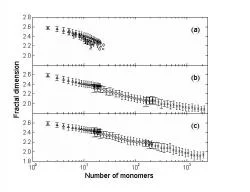
Figure 2. The fractal dimensions given by the Hausdorff dimension. Fractal dimensions for like charged (a), neutral (b), and oppositely charged (c) particles are shown. The first generation is shown with triangles, the second with circles, and the third generation is marked with diagonal crosses.
Aggregate Charging
The conservation model charges ranged linearly from an average of q = 6.9×10 16 C for an aggregate consisting of two monomers to an average of q = 8.3×10 15 C for 21 monomers. The difference between the monopole moments of the two charging methods was examined by plotting the ratio of the charge in the OML model to the charge conservation model (Figure 3). Alternatively, this graph can be said to contain the percentage of the original charge remaining on the grains after a certain number have coagulated under the OML model. It can be seen that the curve fits a power law relationship.
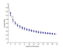
Figure 3. The ratio of the total charge given by OML line of sight to the total conserved charge. The ratio follows a decreasing power law, indicating that as the aggregate grows, a larger proportion of the initial charge is lost.
article_933_order_9
(Equation 24)
Q0 is the original total charge of the constituent grains, N is the number of monomers, and α is calculated to be -0.4988, or about -½. This curve is plotted on top of the data. The magnitudes of the dipole moments were also compared as a function of the number of monomers (Figure 4). It is approximately a linear relationship, but it is plotted on a semi-log graph so that the different scales can be seen. The solid lines indicate the mean value of the magnitude. The mean OML dipole magnitude for a given monomer number is approximately 7.0±1.2% of the mean charge conservation dipole. The ratio only falls from 7.2% for the first half of the data (smaller aggregates) to 6.8% for the second half of the data (larger aggregates), so the ratio is nearly constant. The orientation of the dipole is close for the first few monomers added, but begins to deviate substantially, increasing to an average of 49˚ for an aggregate of 20 monomers. The surface potential as defined by the monopole charge and the radius of maximum extent was plotted (Figure 5). It can be seen that the charge conservation potential continues to rise steadily, while the OML potential falls from -1 V to an equilibrium value around -0.5 V.
article_933_order_11
Conclusions
According to the Hausdorff calculation of the fractal dimension, the fractal dimension decreases with the size of the aggregate. Using the spherically averaged density to calculate the fractal dimension assumes that the fractal dimension is constant within the population. If the fractal dimension decreases with size, then the spherically averaged density will decrease faster than it would if the fractal dimension were constant. This means γ will be artificially low, causing the spherically averaged density method fractal dimension to be lower than the Hausdorff method fractal dimension. Unfortunately the Hausdorff dimensions were calculated with a resolution of one 200th of the aggregate size, which was smaller than the grain size for all but the largest aggregates. Since the grain size gives the lower limit of the validity of the fractal dimension, most of the aggregates were too small to be analyzed accurately with this method. Both methods point to flaws in the other. Which one is correct depends on the application. If it is used to determine how well the space inside the fractal is filled, the Hausdorff is probably more appropriate, whereas if the fractal dimension is used to predict the mass or number of monomers required to reach a given radius, the spherically averaged density is probably better.
article_933_order_12
The OML line of sight approximation gives a reasonable approximation of the charge on a dust aggregate due to primary currents. There are a number of limitations. First, it does not include secondary electron charging. Second, it currently assumes a Coulomb potential, which becomes poorer as the plasma density or particle size increases. Third, the line of sight assumption slightly underestimates the charge. For example, in an aggregate consisting of two negatively charged spherical dust grains, the ions will be attracted, and the electrons will be repelled. This means that the first monomer will block fewer electrons and more ions from reaching the second monomer than predicted by the line of sight model. Consider a particle that just grazes both dust grains (Figure 6). This gives a ring of points on one dust grain where the other grain begins to block the charging currents. This ring is in different places for oppositely charged currents, and the region outside this ring where full charging occurs will be smaller for the oppositely charged current. Thus the OML line of sight slightly underestimates the magnitude of the charge on a particle, but should be a better approximation than charge conservation. In addition, the portion of the original charge which is retained fits closely to the -½ power of the number of monomers, which means it may be possible to model the charge on an aggregate without resorting to the extensive calculations required by the OML line of sight method.
article_933_order_13
The conservation of charge prevents like charged aggregates from growing to a substantial size in (Matthews, Hayes, Freed, and Hyde 2006). The OML line of sight method shows that the rising surface potential which prevented coagulation was not realistic. The surface potential actually falls slightly, allowing increased coagulation. In addition, because the monopole term decays substantially while the dipole term does not, the dipole effects, which promote coagulation (Matthews and Hyde 2004), begin to have a larger effect as aggregate size increases. Therefore OML line of sight shows how coagulation can be more plausible than previously believed.
Acknowledgements
I would like to thank my advisor Lorin Matthews for her assistance and availability, my partner Michael Freed for his consistency, the program director Truell Hyde for his approval, and Keith Walker for informing me of this opportunity. This research made possible by NSF grant PHY-0353558.
References
Blum, J. and G. Wurm. (2000) Experiments on sticking, restructuring, and fragmentation of preplanetary dust aggregates. Icarus 143, 138-146.
Bringol, L. A. and T. W. Hyde. (1997) Charging in a dusty plasma. Advances in Space Research 20(8), 1539-1542.
Chokshi, A., A. G. G. M. Tielens, and D. Hollenbach. (1993) Dust coagulation. The Astrophysical Journal 407, 806-819.
Chow, V. W., D. A. Mendis, and M. Rosenberg. (1993) Role of grain size and particle velocity distribution in secondary electron emission in space plasmas. Journal of Geophysical Research 98(A11), 19065-19076.
Goldstein, H., C. Poole, and J. Safko. (2002) Classical Mechanics: Third edition. 518-519. San Francisco: Addison Wesley.
Haghighipour, H. (2005) Growth and sedemintation of dust particles in the vicinity of local pressure enhancements in solar nebula. Monthly Notices of the Royal Astronomical Society 362, 1015-1024.
Horányi, M. (1996) Charged dust dynamics in the solar system. Annual Review of Astronomy and Astrophysics 34, 383-418.
Horanyi, M. and C. K. Goertz. (1990) Coagulation of dust particles in a plasma. The Astrophysical Journal 361, 155-161.
Kennedy, R. V. and J. E. Allen. (2003) The floating potential of spherical probes and dust grains. II: Orbital motion theory. The Journal of Plasma Physics 69(6), 485-506.
Laframboise, J. G. and L. W. Parker. (1973) Probe design for orbit-limited current collection. The Physics of Fluids 16(5), 629-636.
Mandelbrot, B. B. (1983) The Fractal Geometry of Nature. New York: W. H. Freeman and Company.
Matthews, L. S., R. L. Hayes, M. S. Freed, and T. W. Hyde. (2006) Formation of cosmic dust bunnies, submitted to IEEE Transactions on Plasma Science.
Matthews, L. S. and T. W. Hyde. (2004) Effects of the charge-dipole interaction on the coagulation of fractal aggregates. IEEE Transactions on Plasma Science 32(2), 586-593.
Ossenkopf, V. (1993) Dust coagulation in dense molecular clouds: the formation of fluffy aggregates. Astronomy and Astrophysics 280, 617-646.
Richardson, D. C. (1995) A self-consistent numerical treatment of fractal aggregate dynamics. Icarus 115, 320-335.
Spitzer, L. (1978) Physical Processes in the Interstellar Medium. New York: John Wiley and Sons.
Weidenschilling, S. J. and J. N. Cuzzi. (1993) Formation of planetesimals in the solar nebula. Editors E. H. Levy and J. I. Lunine. Protostars and Planets 1031-1060. Tucson Arizona: The University of Arizona Press.
Wurm, G. and J. Blum. (1998) Experiments on preplanetary dust aggregation. Icarus 132, 125-136.