
Authors: Chathuri N. Wickramaratne, Emily N. Sappington, Hanadi S. Rifai
Institution: Civil and Environmental Engineering, University of Houston, 6100 Main St, Houston, TX 77005
ABSTRACT
The confocal laser fluorescence microscope (CLFM) enables viewing fluorescing objects and creating 3D images by optical sectioning. The CLFM can potentially be used to view, count, and analyze oil droplets, which have naturally fluorescing properties, by image processing techniques. However, many factors, including sample oil concentration, number of optical sections per stack, quantity and location of stacks, and threshold value for grayscale to binary image processing affect the intensity of fluorescence in the images produced and the oil concentration that is calculated. This study aims to establish patterns between these variables and a methodology to accurately calculate oil concentrations. A representative sampling strategy using a grid was developed in this study that allowed the stacks to be evenly obtained across the flow channel, and a total of 60 image stacks were obtained for each sample with varying the z-step size and stack location. A MATLAB code was developed to analyze the image files and calculate the concentration of oil in each sample. The potential applications for this research include viewing fluorescent oil droplets in water discharged from subsea oil and gas production. This technique could be used to demonstrate compliance with subsea-produced water discharge regulations.
INTRODUCTION
The confocal laser fluorescence microscope (CLFM) enables viewing fluorescing objects in samples and creating 3D images by optical sectioning. The study by Wilson (2011) showed that the function of the CLFM is similar to that of a conventional wide-field optical microscope, but the confocal uses spatial filtering techniques to reduce information from the background, rendering higher quality images. The study demonstrated that the CLFM has the capability to eliminate secondary fluorescence from areas outside of its set focal plane by allowing light to pass only through a pinhole. The 3D images are produced in stacks that are a compilation of optical sections which are lateral images of the cross-sectional area of the specimen at each particular point on the z-axis.
The predominant application of the CLFM since its introduction has been in life sciences. However, recent novel studies are investigating the feasibility of CLFM for subsea applications (subsea engineering refers to oil and gas extraction from oceanic environments); more specifically, testing for compliance with discharge regulations by measuring the oil in post-treatment produced water. The microscope can potentially be used to view, count, and analyze the oil droplets in treated produced water to estimate the concentration of oil in a particular sample. Such calculations can be done by image processing techniques to interpret the stacks. Calibration of the CLFM method involves comparison of estimated oil content with the CLFM to a prepared sample with known oil content. This normalized comparison refers to the percent recovery (CLFM estimated content/known content) and the standard deviation of the percent recovery to assess accuracy and precision, respectively.
Several settings on the CLFM affect the intensity of the fluorescence in the images produced, and thus, affect the concentration of oil that is calculated. One study utilized the CLFM for geochemical analysis of cave deposits and addressed this issue of fluorescence intensity by maintaining all settings constant in an effort to normalize the fluorescence intensity measurements (Orland et al., 2014). None of the previous studies with CLFM, however, have delineated a clear relationship between a sample oil concentration, the number of optical sections per stack, the quantity and location of stacks, the percent recovery, and the standard deviation. This is largely due to the lack of a systematic method in retrieving confocal image data.
The objective of this research is to establish a strategy for representative sampling and identify patterns between the sample concentration, number of optical sections per stack, quantity and location of stacks, threshold value for grayscale to binary image processing, percent recovery, and standard deviation. This research proposes that the percent recovery and standard deviation from the CLFM data are dependent on the sample concentration, the number of stacks, the number of optical sections per stack, and threshold value. Elucidating the inherent relationships among the aforementioned variables would lend rigor and a higher degree of confidence with the CLFM method and would expand its use beyond life sciences into environmental and water quality applications.
MATERIALS AND METHODS
Sample Preparation
Samples of synthetically produced water were prepared using crude oil (specific gravity: 0.908mg/L; API gravity: 24.3˚) from an onshore facility (undisclosed location) in Millipore water (U.S. Filter Modulab Water Systems MAU 149 96023, U.S. Filter Coporation) at concentrations of 15, 25, 30, 40, 50, 100, and 500ppm. Using the density relationship, a known mass of crude oil was transferred into amber glass bottles with PTFE-lined caps using a Pasteur pipette; known as the weight by difference technique (Supplementary Figure S1). Each sample was mixed using a homogenizer (IKA T 18 digital Ultra-Turrax, North Carolina, U.S.) for one hour at 12,000 Revolutions Per Minute (rpm) before being injected into the flow cell (Ibidi µ-Slide 0.4 Luer ibiTreat #1.5 polymer coverslip, tissue culture treated, sterilized, Focus, Germany) (Supplementary Figure S2 and S3). Initially, samples were injected into the flow cell using a gastight glass syringe with a PTFE-lined plunger, but this technique resulted in uneven droplet sizes and poor distribution throughout the flow cell (Supplementary Figure S4). A Pasteur pipette was then tested and used for the experiments, which improved the homogeneity of oil droplets within the flow channel (Supplementary Figure S5).
Flow Cell Sampling Methodology

Figure 1. Grid for representative sampling.
To ensure representative sampling of the stacks from the flow cell, a grid was constructed by soldering metal wires together and placed over the flow cell on the microscope stage (Figure 1). The grid divided the flow cell channel area into 12 cells (numbered 1 to 12), each with dimensions of 2mm x 7.5mm x 0.4mm (Figure 2). The length and width were measured manually and the depth is the depth of the flow channel provided by Ibidi. For each sample injected into the flow cell, 5 stacks of images were taken at identical locations within each of the 12 cells with varying z-step size of 2, 4, 6, 8, and 10µm resulting in a total of 60 0.4mm-height stacks.
Confocal Laser Fluorescence Microscope Settings

Figure 2. Divsion of flow channel into grid cells. The flow channel runs through the center of flow cell and is 400μm deep. The metal grid divided the channel area into 12 cells that were approximately 2mm x 7.5mm each. Each cell was assigned a number, as indicated in the figure, which was later used when randomly selecting stacks taken from the sample for an averaged calculation of the crude oil concentration.
Several settings on the CLFM software (Leica DM2500B SPE confocal, Leica Microsystems, Germany) were determined before obtaining the stacks (Supplementary Figure S6). The gain for the photomultiplier tube (PMT) was set to 800. The gain ranges from 1 to 1250 and functions similarly to the exposure of a camera. However, since the brightness of the images produced depends on both the gain and the intensity of the laser with a multiplication effect, the gain was held constant for all experiments and laser intensity was adjusted for each individual stack. Since oils are typically excited by wavelengths ranging between 300nm and 400nm, the 488nm laser was used on the CLFM because it was closest to known oil excitation wavelengths (Karpicz et al., 2005; Steffens, Landulfo, Courrol, & Guardani, 2010). Grayscale images were obtained using the Leica CLFM software, with the shades of gray range from 0 to 255 where 0 is a black pixel, 1 is white pixel, and 1 to 254 are pixels of various shades of gray. The “quick LUT” icon on the Leica CLFM software displays the image pixels in a color gradient from yellow to blue (instead of grayscale) based on the emission intensity of the region which helps facilitate viewing the spectral range of the image (Supplementary Figure S7). To ensure that the full spectral range of each image is utilized, the laser intensity was adjusted so that some blue pixels were visible in the display, which represent the brightest pixels (shade number 255) and indicate that the brightest emissions were displayed with maximum intensity in the captured image. The shortest wavelength of the emission spectrum was set to 500nm which is 10 to 15nm higher than the excitation wavelength to prevent interference patterns in the image (Karpiczet al., 2005).
Data Processing
A MATLAB (R2014a) program was developed to process the image stacks acquired from the confocal microscope and calculate the concentration of oil in the sample. The code first converts the grayscale images into binary images using a threshold value that determines whether a grayscale pixel is converted to a white or black pixel based on its magnitude. The code tested threshold values ranging from 0.05 to 0.95 in increments of 0.05 and calculated the oil concentration at z-step sizes of 2, 4, 6, 8, and 10µm for each stack of images. An optimal threshold value was identified for each z-step based on which threshold value yielded the concentration with the least sum squared error with respect to the known (prepared) concentration of the sample. The MATLAB’s built-in randomization function was used to select 3, 6, 9, and 12 calculated concentrations from the 12 possible grid cells, and then the selected concentrations were used to determine the average oil concentration at the optimum threshold. Based on these concentration calculations, the percent recovery and the standard deviation were calculated (Equation 1 and 2, respectively, see PDF).
Comparison to EPA 1664
Treated produced water is tested via EPA Standard Method 1664 (USEPA, 2010) to ensure that its oil content meets acceptable discharge criteria. The same acceptability criteria used in EPA 1664 were adopted in this study. Thus, for each sample, the criteria for initial precision and recovery performance tests from EPA 1664 (83-101% percent recovery, ≤11% standard deviations) were used as a guideline for acceptable percent recoveries and standard deviations in the experiments presented in this research.
RESULTS
The resulting standard deviations and percent recovery values for the CLFM experiments are indicated in Table 1. The highlighted values indicate acceptable percent recoveries and standard deviations using EPA 1664 guidelines. Many of the concentrations show acceptable percent recoveries, especially when more stacks were used for the calculation, but most of the standard deviations did not meet these criteria. The optimum thresholds calculated for 15, 25, 30, 40, 50, 100, and 500ppm samples were 0.4, 0.3, 0.4, 0.3, 0.35, 0.3, and 0.3, respectively. Overall, little to no correlation between z-step size and percent recovery was identified, but a positive correlation between number of stacks and percent recovery was observed.


Table 1. Percent recoveries and standard deviations of all tested sample concentrations. Z is the z-step used when acquiring image stacks, which describes the increments between each optical section within the image stacks. Recovery (%) is the CLFM estimated concentration divided by the prepared sample concentration multiplied by 100% (Equation 1). Standard Deviation (%) is the deviation of the CLFM calculated concentration of a stack from the average calculated concentration (Equation 2). The highlighted values indicate acceptable percent recoveries and standard deviations as stated in the criteria for initial precision and recovery performance tests from EPA Standard Method 1664 (USEPA 2010).

Figure 3. Percent recovery versus z-step and number of stacks for 15 ppm sample. Little to no correlation is evident for percent recovery with respect to z-step, but it is apparent that percent recovery is decreasing with increasing number of stacks for this 15ppm crude oil sample.

Figure 4. Percent recovery versus z-step and number of stacks for 25 ppm sample. No correlation is evident between percent recovery and z-step size, but a somewhat parabolic relationship is displayed in this 25ppm crude oil sample for percent recovery with respect to number of stacks used.
The 15ppm sample yielded acceptable percent recoveries using six cells for z-steps 4, 6, 8, and 10µm that ranged from 84.5% to 87.1%. The standard deviations of the percent recoveries ranged from approximately 22% using nine cells for a z-step of 6µm to 112% using three cells for a z-step of 2µm, which do not meet the acceptable criteria. No strong correlation was observed between z-step size and percent recovery and a negative correlation between number of stacks and percent recovery was observed (Figure 3).
The 25ppm sample yielded acceptable recoveries ranging from 98.9% to 101.0% from using 12 cells for all z-steps and using nine cells for z-steps of 8 and 10µm. No acceptable standard deviations were observed across all z-steps and ranged from approximately 17% to 46%. Again, no strong correlation between z-step size and percent recovery was observed. The lowest percent recoveries occurred using six cells, displaying a somewhat parabolic trend between the number of stacks and percent recovery (Figure 4).

Figure 5. Percent recovery versus z-step and number of stacks for 30 ppm sample. The 30ppm crude oil sample showed increasing percent recovery with increasing number of stacks used but no strong correlation with z-step size.
The 30ppm sample had acceptable recoveries from 83.0% to 85.5% for six cells and z-step size of 2, 4, 6 and 8µm, nine cells and z-step size of 2, 4, and 6µm, and 12 cells for a z-step size of 2µm. Standard deviations ranged from approximately 12% to 33%, none of which were acceptable. The percent recovery increased with increasing number of stacks and no strong correlation was evident between z-step size and percent recovery (Figure 5).

Figure 6. Percent recovery versus z-step and number of stacks for 40 ppm sample. The 30ppm crude oil sample showed increasing percent recovery with increasing number of stacks used but no strong correlation with z-step size.
The 40ppm sample yielded acceptable percent recoveries ranging from 83.2% to 100.0% for using six cells at all z-step sizes and using three cells at z-step sizes of 2, 4, 6, and 10µm, and using nine cells for a z-step size of 6µm. The standard deviations observed ranged from 19.7% to 31.3%, none of which were acceptable. No strong correlation between z-step and percent recovery was observed. Percent recovery increased with number of stacks used (Figure 6).

Figure 7. Percent recovery versus z-step and number of stacks for 50 ppm sample. The 50ppm crude oil sample yielded higher percent recoveries with increasing number of stacks and showed no strong correlation between percent recovery and z-step size.
The 50ppm sample yielded acceptable recoveries for all z-step sizes using 6, 9, and 12 cells that were from 88.0% to 97.7%. Again, no acceptable standard deviations were observed, ranging from 15.6% to 36.7%. No strong correlation between z-step size and percent recovery was observed. Percent recovery increased with an increasing number of stacks used (Figure 7).

Figure 8. Percent recovery versus z-step and number of stacks for 100 ppm sample. The 100ppm sample yieled results that were relatively consistent across all z-steps, suggesting no strong correlation with percent recovery and increasing percent recovery with increased number of stacks used.
The 100ppm sample had acceptable recoveries that ranged from 98.6% to 101.0% using three cells for z-step sizes of 2, 4, 6, 8µm and using six cells and a z-step size of 2 and 6µm. Acceptable standard deviations of 6.9% to 10.0% were observed using three cells for z-step sizes of 2, 6, 8, and 10µm. There was no strong correlation between z-step size and percent recovery, and an increase in percent recovery with an increase in number of stacks used was observed (Figure 8).
The 500ppm sample gave acceptable percent recoveries using 9 and 12 cells for all z-steps ranging from 88.9% to 97.9%. The observed standard deviations ranged from 12.0% to 21.3%, none of which were acceptable. The percent recoveries slightly decreased with increasing z-step size and generally increased with increasing number of stacks used (Figure 9).

Figure 9. Percent recovery versus z-step and number of stacks for 500 ppm sample. The 500ppm sample showed results that had slightly decreasing percent recovery with increasing z-step size and highest
DISCUSSION
Overall, the results indicated that all samples had relatively symmetric graphs along the z-step axis, suggesting that concentration does not depend strongly on the z-step size used. Since a shorter amount of time is needed for the CLFM to obtain stacks with increasing z-step size, it may be more efficient to use larger z-steps, while still retrieving accurate concentration calculations (Supplementary Table S1). However, further studies can be conducted to assess the upper limit of acceptable z-step size since the experiments in this study defined a scope of testing up to a z-step of 10m.
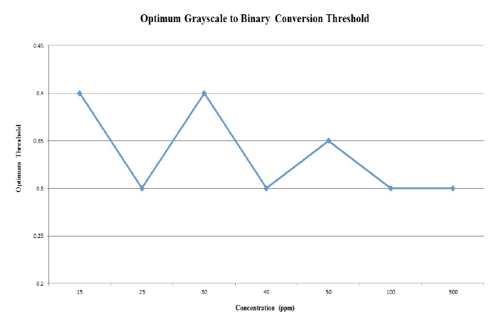
Figure 10. Threhold versus sample concentration. The optimum grayscale to binary threshold identified for the various concentrations of crude oil samples are relatively consistent and average approximately 0.33.
The optimum threshold values as determined using the MATLAB code were between 0.3 and 0.4 for samples ranging from 15ppm to 500ppm of crude oil, which is relatively consistent for such a wide distribution of sample concentrations (Figure 10). Thus, for future experiments using the same type of crude oil, the average threshold value of approximately 0.33 may be sufficient for comparable results. Experiments were performed using 10ppm crude oil, but oil could not be visualized through the CLFM to obtain results, suggesting that such concentrations are approaching a lower limit. It should be noted that this threshold range may only be applicable for the specific crude oil type used in these experiments for reproducible results.
Although the homogeneity of the crude oil-water solution within the flow cell improved with the change in injection equipment (Pasteur pipette instead of syringe), it was not enough to yield accurate calculations using the random sampling technique of the flow cell area since this technique is not ideal until homogeneity within the flow channel can be established. The original purpose of testing the effect of using 3, 6, 9, and all 12 stacks taken from the sample using the grid cells was in pursuit of a finite number of stacks that would yield a comparable concentration to circumvent sampling the entire flow cell. If a smaller number of stacks can be sampled to yield a similar concentration calculation, then less time would be needed to achieve the calculation, which would be a financial incentive to energy producers in oil and gas operations. However, this was not the case in these experiments since different areas of the flow cell contained different concentrations of oil. Thus, random selections of stacks yielded highly variable concentration calculations that required more sampling to get better representation of the concentration.
The issue of heterogeneity is reiterated by the large standard deviations of the percent recoveries observed consistently across all of the experiments conducted. Although the average concentration of the stacks took yielded values close to the prepared concentration value, the calculations were often offset by outliers from some stacks. Several experiments had results showing lower standard deviations using three stacks because the randomly selected stacks used were similar in value, by chance, as determined by the randomization function in MATLAB. Using three stacks for concentration calculation, although providing acceptable results several times, is highly inconsistent because it is by chance that it is representative or misrepresentative of the sample concentration. On the other hand, the standard deviations of percent recoveries using 12 stacks were consistently higher and unacceptable. It can therefore be noted that the standard deviation values are not representative of the precision in using a greater number of stacks since it only exemplifies the heterogeneity of the oil throughout flow cell area.
Due to the obstacle of heterogeneity presented by these experiments, further studies must be conducted to produce a more homogenous distribution of oil droplets within the flow cell so that a random sampling technique can be utilized with a smaller number of stacks needed to yield an accurate calculation of the concentration. Alternatively, efforts to maximize the number of stacks taken must be made so that the flow cell can be more representatively sampled using a technique similar to that presented in this study.
Based on the findings from this study, it can be concluded that CLFM is a promising technology for detecting oil in water, especially if homogeneity in oil distributions within the treated effluent can be ensured. This is likely to be the case in closed subsea systems whereby the produced water can be treated and tested inline or offline under relatively high velocities that maintain a well-mixed sampled matrix.
ACKNOWLEDGMENTS
Dr. Charisma Lattao, Jingjing Fan, and Amin Kiaghadi are acknowledged for their guidance and assistance throughout the project.
REFERENCES
Karpicz, R., Dementjev, A., Z., Kuprionis, S., Pakalnis, R., Westpahl, R., Reuter, R., & Gulbinas, V. (2005). Laser Flourosensor for Oil Spot Detection. Lithuanian Journal of Physics, 45(3), 213-218. doi:10.3952/lithjphys.45309
Orland, I. J., Burstyn, Y., Bar-Matthews, M., Kozdon, R., Ayalon, A., Matthews, A., & Valley, J. W. (2014). Seasonal climate signals (1990–2008) in a modern Soreq Cave stalagmite as revealed by high-resolution geochemical analysis. Chemical Geology, 363, 322-333. doi:10.1016/j.chegeo.2013.11.011
Steffens, J., Landulfo, E., Courrol, L. C., & Guardani, R. (2010). Application of Fluorescence to the Study of Crude Petroleum. Journal of Fluorescence, 21(3), 859-864. doi:10.1007/s10895-009-0586-4
U.S. Environmental Protection Agency. (2010). Method 1664, Revision B: n-Hexane Extractable Material (HEM; Oil and Grease) and Silica Gel Treated n-Hexane Extractable Material (SGT-HEM; Non-polar Material) by Extraction and Gravimetry. Office of Water (4303T), 1200 Pennsylvania Avenue, NW, Washington, DC 20460. EPA-821-R-10-001.
Wilson, T. (2011). Resolution and optical sectioning in the confocal microscope. Journal of Microscopy, 244(2), 113-121. doi:10.1111/j.13652818.2011.03549.x