

Authors: Julia Mareli Sanchez, Terry Ferguson, & Kaye Savage
Institution: Department of Encironmental Sciences and Department of Biology, Wofford University, 429 N Church St, Spartanburg, SC 29303, USA
Date: October 2017
doi:10.22186/jyi.33.4.90-98
Abstract
Seasonal floodplain wetlands occur throughout the Piedmont Region of South Carolina, providing a plethora of ecosystem services. As a result of extensive soil erosion during the agricultural period from mid-1700s until mid-1900s, Piedmont floodplains have accreted significantly, altering their natural flood regime. The purpose of this study was to better understand the impacts of land use change and seasonality on the hydrology of two adjacent, seasonal floodplain wetlands. This was done by evaluating water levels in each wetland for a period of twelve months using wells, monitoring groundwater through a piezometer, characterizing sediments from 0 to 21cm, and comparing rainfall events to the Lawson’s Fork Creek stream gage and wetland water levels. It was found that the type and intensity of rainfall events were key components driving wetland water level changes during each season. During storm events, the wetlands aided in flood control; results show that they may be hydraulically connected during intense overbank flooding events. Groundwater was not found to recharge the surface during dry periods, as proposed, which could be due to low sample size and only one piezometer. The results of this study demonstrate the need for long term hydrological research of small seasonal wetlands in order to better protect and manage the ecological services they provide.
Introduction
Wetlands are a common feature in floodplain ecosystems and are known to aid in flood control, act as land buffers to prevent erosion, improve water quality by filtering nutrient-laden sediments, and provide a habitat for unique species of plants and animals (Welsch et al., 1995; Yu et al., 2015). They are also important breeding sites for amphibians and critical foraging locations for reptiles and birds (Semlitsch, 2008; Yu et al., 2015). Since they are found in transitional areas between aquatic and terrestrial ecosystems, floodplain wetlands are largely influenced by rivers and streams (Tockner and Stanford, 2002). Ecological communities that depend on these wetlands are limited by their ability to live in seasonally saturated conditions and are directly impacted by the dynamic hydrology of the wetlands. Since the wetland’s hydrology dictates its ecology, soil type, and community composition, understanding the processes that drive water level changes in these areas is crucial for developing management strategies of watersheds that contain wetlands (Stratman, 2002). More research that solely focuses on the hydrology of floodplain wetlands is needed to supplement and enhance what is already known biologically (Connor & Gabor, 2006).
In contrast to other wetland types such as glacial or coastal wetlands, fluvial or floodplain wetlands tend to have hydroperiods that correspond to stream discharge (Kirkman et al., 1999). A hydroperiod is a seasonal pattern of surface water levels that affects the storage capacity and the water budget of the wetland; they are directly influenced by precipitation, the area’s microtopography, and surface-groundwater interactions (Welsch et al., 1995; Yu et al., 2015). Since hydroperiods drive the biota and biogeochemical processes of a wetland, it is important to characterize and monitor them seasonally (Kingsford, 2000; Kirkman et al., 1999).
Seasonal floodplain wetlands occur throughout the Piedmont Region of South Carolina (Yu et al., 2015). They are characterized by their small area, depressional topography, and shallow depth (Hayashi & van der Kamp, 2000). Although the geomorphic origin of floodplain wetlands varies throughout the world, land use changes tremendously impact a region’s topographical character and function (Pitt et al., 2012). Extensive soil erosion during the agricultural period, from mid-1700s until mid-1900s, had caused the Piedmont floodplains to accrete significantly with an average of 1m to 2m (Happ, 1945). This accumulation of deposited sand and micaceous sandy silt has altered the area’s microtopography and natural flood regime (Happ, 1945).
Such is the case with the Lawson’s Fork creek, a third order stream that discharges into the Pacolet River downstream of Glendale, South Carolina (USGS-SC #02156300). Glendale was the location of the earliest textile mill in this region of the Piedmont and operated from 1832 to 1960. Historic Records indicate that a dam was present at Glendale since the 1830s. After the mill ceased its operation in 1960s, the dam was no longer regulated. Over time, the 22.3-hectare mill pond has been filled in with deltaic sediments, initially transforming the mill pond into a network of distributary channels and islands, which were eventually filled in to become a forested floodplain with seasonal wetlands.
Two neighboring, seasonal wetlands in the Lawson’s Fork floodplain, named Beaver and Dragonfly for the purpose of this study, have an observable impact in the area ecologically. However, little is known about their hydrology. Beaver wetland measured 1.9 acres in area in May 2015, and is depressed 0.6m below the surrounding floodplain. An ephemeral stream on the north side of the wetlands feeds it during inundated conditions. Vegetation is seasonally variable, consisting mainly of water starworts and duckweed in the winter months, and blue joint grass, broadleaf arrowhead, wild proso millet, nut grasses and marsh ferns in the spring/summer months. Scattered hardwood deciduous trees, such as river birch and sweet gum, persist year-round. Dragonfly wetland measured 2.35 acres in May 2015. Seasonal vegetation is similar to that described for Beaver wetland.
Small fluvial wetlands like Beaver and Dragonfly are largely overlooked and understudied, in part due to their small size, the difficulty associated with their delineation, and their transient nature (Pitt et al., 2012). Previous research on seasonal floodplain wetlands has focused on understanding their roles in water quality and purification, their potential as a habitat, and the pertinence of including them in conservation legislation (Coleman, Diefenderfer, Ward, & Borde, 2015; Pitt et al., 2012; Yu et al., 2015). Few studies have focused solely on their hydrology. Thus, the purpose of this study was to better understand the impacts of land use change and seasonality on the hydrology of the area. Our main objective was to observe the response of Beaver and Dragonfly to rainfall events and groundwater, and to evaluate the seasonal patterns of inundation and subsequent water efflux over a twelve-month period. Due to the geographical proximity between Beaver and Dragonfly, we proposed that their water levels would fluctuate similarly in response to temperature changes and storm events. We also expected the groundwater to recharge the surface during seasonally dry periods. Through analysis of wetland water levels, stream gage readings for storm events, groundwater monitoring, and sediment characterization, this study provides key baseline data for the long-term management of these riverine wetlands, and other riverine wetlands around the world. A recent study in Southeast Australia found that floodplain wetlands could act as long-term sinks of atmospheric carbon, suggesting that they may play a role in alleviating the effects of climate change by sequestering CO2 (Kobayashi, Ralph, Ryder, & Hunter,2013). Proper management of seasonal floodplain wetlands and a thorough understanding of their hydrological regime could enhance their function as a sink for CO2, and as critical hubs for biodiversity. Understanding their hydrology is a crucial step towards creating a comprehensive plan to ensure their future survival. Locally, the Spartanburg Area Conservancy is currently building a hiking trail adjacent to the Lawson’s Fork Creek and the two wetlands. The findings of this study will have a direct impact on the management of the area by restricting trail usage when heavy storms are expected to hit the watershed, thus contributing to the trail’s success and the safety of the hikers.
Methods
Field Site
This research was conducted in the Lawson’s Fork Creek watershed in Glendale, SC (34.9450° N, 81.8364° W). The Lawson’s Fork feeds into the Pacolet River in the upstate of South Carolina (Figure 1). The study site contains two neighboring wetlands, named Beaver and Dragonfly for the purpose of this study. They were chosen due to their size, proximity to the Lawson’s Fork creek (Figure 1), and their location downstream of a USGS stream gage (USGS #02156300). The wetland downstream and closest to Glendale was designated as “Beaver,” while the wetland upstream was designated as “Dragonfly” (Figure 1).

Figure 1. ESRI generated map of Lawson’s Fork Creek and the town of Glendale. The red mark indicates the location of the USGS stream gage (USGS #02156300). The blue marks indicate the location of the neighboring wetlands, designated as Beaver and Dragonfly for the purpose of the study. Map of South Carolina in bottom right corner indicates the location of Spartanburg County.
In this study, the Army Corps of Engineers’ definition of a wetland was used. It is defined as an area inundated or flooded by surface or groundwater that supports vegetation and fauna adapted to saturated soil conditions (Corps of Engineers Wetlands Delineation Manual, Technical Report Y-87-1, 1987). This definition was chosen because it is used by the Clean Water Act for regulatory and management purposes. However, due to the dynamic nature of the wetlands’ hydroperiod, delineating a specific boundary for each wetland was difficult. The functional boundaries used in this study were delineated when standing water was present in May of 2015, and the boundary was defined at the edge of the ponded water. Thus, the wetland boundary may be an underestimate. The Fish and Wildlife Service (FWS) delineation of the area was used as a template boundary (Figure 2). Google Earth Pro was used to plot waypoints on the FWS map, then those points were ground-truthed by physically walking the wetland perimeter. If the waypoint on the FWS map matched the boundary of standing water in the field, then it was recorded as “present”. If the waypoint was not accurate, it was marked as “absent” and the GPS coordinates were recorded at the observed water boundary (Figure 2).

Figure 2. Google Earth map derived from Fish and Wildlife Service wetland delineation database. Yellow outline represents area of Glendale Mill pond in 1921. Turquoise area represents delineated outer boundary of wetlands, based on FWS delineation. Circle on the right refers to the Beaver Wetland, circle on the left refers to the Dragonfly wetland.
Wells and Piezometer
To monitor the water levels, a PVC pipe which is 1.5m in length, 2.54cm in diameter, and screened all the way to the top was installed in each wetland. The wells were protected by a synthetic sock to keep out plant material and fine sediments. Both wells were implanted into roughly 1m of sediment. Each well was equipped with a water level logger (Solinist Canada Ltd., Ontario) hanging from a metal wire attached to a metal cap. A barometric pressure logger (Solinist Canada Ltd., Ontario) was installed on a nearby tree in Dragonfly wetland, approximately 5m away from the well, to monitor the surrounding air pressure. Water level and barometric pressure data were collected from May 29, 2015 to May 14, 2016 at 15-minute intervals. The water level data were downloaded and compensated for pressure using Solinist Levelogger software. Water level was measured in meters to the nearest hundredth. A Welsch two sample t-test was used to determine the differences in water level means. Test was performed using R software.
Rainfall data was collected at the Glendale weather station, and analyzed for 2015 and 2016. Total rainfall in each month was plotted and compared in a bar graph (Figure 3). Gage height data from a major storm event in October 2015 were extracted from the USGS stream gage database. The data were compared to the water levels in each wetland during a four-day storm event, from October 2 to October 6, 2015, and a Welsch two-sample t-test was performed in R.
A piezometer was installed at a depth of 2m in the Dragonfly wetland (Solinist Canada Ltd., Ontario). Piezometers measure the pressure head of groundwater at a specific point. In relation to other water level measurements, they indicate the direction of groundwater flow (Dodds & Whiles, 2010). Piezometer water levels were monitored in relation to the well in Dragonfly, and the direction of groundwater flow was determined. Water levels were measured manually using an electric water level meter six times between May and October of 2015 (Solinist Canada Ltd., Ontario). For analysis, the times when water levels were recorded in the piezometer were matched to the closest 15-minute interval in the well water level logger. Statistical analysis of water levels and piezometer readings was performed in R.
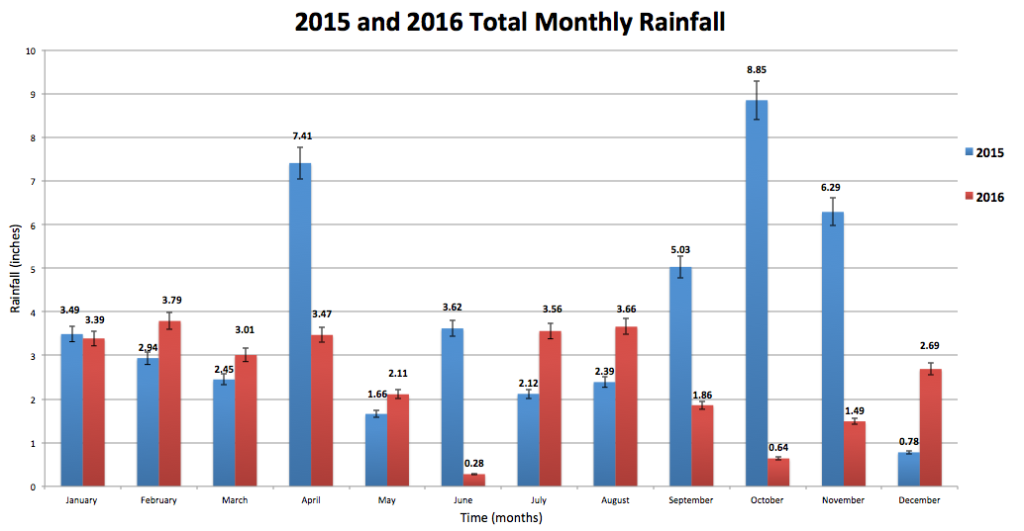
Figure 3. Total monthly rainfall in 2015 and 2016. Data extracted from the Glendale weather station. Numbers above bar show total monthly rainfall, and error bars show standard error. Data reported in inches.
Sediment Analysis
Due to hunting season restrictions, only a single sediment sample was collected in the Beaver wetland using a universal core head sediment sampler (WaterMark®, Canada), chosen because it is specifically designed for saturated, fine sediments. A total of 0.55m of sediment was recovered. The sediments were separated into four observable segments (or depositional layers), weighed, and dried for 3 days. A LaMotte Soil Texture Kit (LaMotte Company, Maryland, USA) was used to determine, via precipitation, the percentage of sand, silt and clay by volume and weight for each segment of the core. The hydraulic conductivity of each segment was then estimated based on a table of values published in Ground and Surface Water Hydrology (Figure 3.7; Mays, 2012).
Results
Wetland Water Levels and the Storm Event in October 2015
Results show that water levels in each wetland fluctuate seasonally in response to rainfall events and temperature changes (Figure 4). While water levels in Dragonfly and Beaver appear to respond similarly to rain events, as shown by the overlapping spikes (Figure 4), mean water levels during the twelve-month period were found to be significantly different (M = 0.52±0.004, SD = 0.411; M = 0.584±0.005, SD = 0.320, p < .001, df = 61448). An inverse relationship was observed between the changes in water levels and the changes in temperature during the year from 2015 to 2016 (Figure 4).

Figure 4. Water level fluctuations (m) and Temperature (C) from May of 2015 to May of 2016. Blue line indicates the Dragonfly wetland, and red line indicates the Beaver wetland water levels (primary vertical axis). Green line indicates Temperature in C (secondary vertical axis).
During the October 2015 overbank-flooding event, wetland’s water level fluctuations reflected the pattern of water level peaks and lows in the stream (Figure 5). Water levels in the wetlands ranged from 0.5m to 0.95m (Dragonfly: M = 0.838±0.004, SD = 0.091; Beaver M = 0.749±0.005, SD = 0.118), while water levels in the stream ranged from 1.5m to 4.5m (M = 2.593±0.038, SD = 0.829). Peak discharge was approximately 13.0ft3/sec (0.37m3/sec) on October 3, which is also the day in which the highest water levels in the well of each wetland were recorded (0.93m in Dragonfly, 0.87m in Beaver). Water levels in the Dragonfly’s well remained higher than those of the Beaver’s well for the duration of the storm event, and their means were significantly different (p < .001) (Figure 5). A significant difference was also found in the mean water levels of both wetlands when compared to the stream gage mean water levels (p < .001) (Figure 5).
Total Monthly Rainfall
October and November were the wettest months of 2015, while February and August were the wettest months of 2016 (Figure 3). October 2015 was unusually wet, with a total rainfall of 8.85in (22.5cm). Total rainfall during the four-day October storm event was 3.35in (8.5cm). October 2016 was unusually dry, with a total rainfall of only 0.64in (1.6cm). No seasonal pattern of rainfall was found between 2015 and 2016.
Piezometer Readings
Water levels in the piezometer were measured six times during the twelve-month study period and compared to the water levels in Dragonfly (Figure 6). When the wetland was ponded, water levels in the Dragonfly’s well were above 0m. It was found that water levels in the piezometer were lower than water levels in the well: 0.75m in the well and 0.63m in the piezometer in June 2015. When water levels in the Dragonfly’s well were either approaching 0m or below 0m, it was found that water levels in the piezometers were higher than the bottom of the dry well, which is 0.02m. No significant differences were found between the wetland and piezometer water levels (M = 0.422±0.169; M = 0.487±0.117; p = .373).
Sediment Analysis
Estimations of the hydraulic conductivities according to amounts of sand, silt and clay in each sediment interval are given in Table 1 (Mays, 2012). The sediment intervals [10-15cm] and [15-21cm], which contained a higher percentage of sand, had the highest hydraulic conductivity. The sediments at the top of the sediment interval and closest to the surface, [0-6cm], were composed mostly of silty clay and is therefore estimated to have a lower hydraulic conductivity (Table 1).

Table 1. Percent sand, silt, and clay for each sediment interval, determined using a LaMotte Soil Texture Unit. The hydraulic conductivities are estimated according to percentages of sand, silt, and clay.
Discussion
Due to the geographical proximity between Beaver and Dragonfly, we hypothesized that their water levels would fluctuate similarly in response to temperature changes and storm events. We also expected the groundwater to recharge the surface during seasonally dry periods. The study suggests that the type, duration, and intensity of rainfall events were key components driving wetland water level changes during each season. Rainfall in 2015 and 2016 varied monthly and no pattern could be deduced, suggesting that rainfall in this area is variable (Figure 3). The October 2015 overbank-flooding event was not repeated in October of 2016, and occurred instead in the early August of 2016 (USGS, NWISD). The ecological community of each wetland depends on this influx of water; differences in timing of annual overbank events directly impact the phenology of the organisms that require a ponded wetland for their ecological need (Pitt et al., 2012). High volume rainfall events that result in overbank flooding carry nutrient-laden sediments that make the soil extremely fertile when deposited in wetlands (Welsch et al., 1995). Seasonal plants are adapted to these highly variable conditions, and their establishment depends on these overbank-flooding events and seasonal rain events (Tockner Malard, & Ward, 2000). Although excluded from this study, rainfall and temperature changes also contribute to the rates of evapotranspiration, which in turn, impact the water levels in each wetland (Kirkman et al., 1999; Yu et al., 2015).
Lawson’s Fork’s stream discharge during the October 2015 storm event exhibited a flashy hydroperiod with characteristic peaks fluctuating up and back down in hours (Figure 5). Although the graph visually depicts that Beaver and Dragonfly water levels are fluctuating similarly, results show that mean wetland water levels are significantly different during the storm event (Figure 5). While we expected wetland water levels to differ from Lawson’s Fork’s water levels, a statistical difference in the mean water levels of Beaver and Dragonfly during the storm event was surprising, and indicates that the wetlands respond differently to over-bank flooding events, which rejects our original hypothesis. Despite their geographical proximity, this difference in response could largely be attributed to the size of the wetlands. Dragonfly has a greater surface area, and thus maintained a higher water level than Beaver during the storm event. A larger basin allows a wetland to store more water, thus increasing its water level over time. A second explanation for why our hypothesis was not supported is the presence of an ephemeral stream north of the Beaver wetland. Ephemeral streams are common in floodplain wetlands, and can act as regulatory mechanisms for controlling the size and extent of a wetland (Junk, Bayley, & Sparks, 1989). Pitt et al. (2012) also found that seasonal wetlands in the Piedmont region are associated with ephemeral or non-permanent streams, and actually confound remote sensing instrumentation. This outflow of water is likely to be contributing to the water level differences during large storm events.
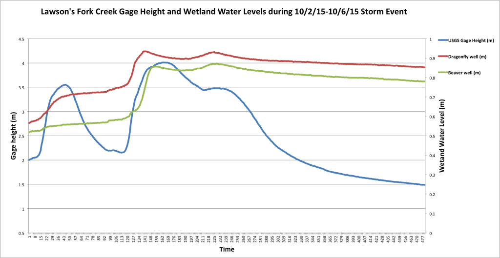
Figure 5. Lawson’s Fork Creek Gage height (m) and wetland water levels (m) during the October 2, 2015-October 6, 2015 storm event. Blue line is the gage height, and peaks reflect the height of the stream at a particular point in time during the event (primary vertical axis). Red line indicates water levels in Dragonfly, and green line indicates water levels in Beaver (secondary vertical axis).
Higher water levels in the Lawson’s Fork creek when compared to the wetlands can be explained by a floodplain wetland’s hydroperiod, which typically tends to be prolonged (Figure 5). Since wetlands act as flood storage basins, they tend to have longer response times and lower peak stormflows (Welcsh et al., 1995). A lower peak in the wetland water levels was observed when compared to the USGS gage height in Lawson’s fork, indicating that Beaver and Dragonfly wetlands aid the floodplain in flood control, and regulate the influx of water during overbank events (Figure 5). A lower peak in wetland water level could also be explained by the area’s depressional topography, which could be slowing down the rate at which water inundates each wetland, causing the peak to culminate at a slower rate.
Beaver’s lower water levels than Dragonfly’s during and after the October 2015 storm event may be due to the presence of an ephemeral stream north of the Beaver wetland. Not only could this stream contribute to the differences in response to storm events, as discussed above, it may also be subsidizing water in Beaver and regulating how much water that can be stored in the wetland. This water outflow may act as a regulatory mechanism for the wetland’s water levels, providing an outlet for flood waters that is not present in Dragonfly wetland (Welsch et al., 1995).
While Beaver and Dragonfly wetlands responded similarly to rainfall events of low intensity, they ponded at different rates after the major storm event in October of 2015 (Figure 4 & Figure 5). Dragonfly ponded rapidly, while Beaver ponded more slowly and maintained relatively lower water levels than Dragonfly after the storm event. One possible explanation is that Beaver and Dragonfly may differ in storage capacity, determined by how well the soils drain and the micro-topography of the area (Welcsh et al., 1995). Dragonfly is at a slightly higher elevation compared to Beaver, so the lag time in Beaver’s inundation could be due to the fact that the wetlands are hydraulically connected. When the Dragonfly wetland reached a certain threshold of inundation, water runs off. This outflow of water becomes the inflow into the Beaver wetland. Since water flows from high to low elevation, the delay in inundation of Beaver could be attributed to this difference in elevation. Beaver’s and Dragonfly’s possible hydraulic connection could have important ecological implications, such as the habitat expansion of aquatic wildlife by creating a channel that allows for movement between wetlands, enhance spore or seed dispersal of plants, and can increase the water’s nutrient availability (Weber, 2012; Welcsh et al., 1995).
Along with surface water dynamics, it was inferred that groundwater played a significant role in the wetlands during seasonally dry periods. While results showed that groundwater levels were higher in the piezometer than in the Dragonfly well when the wetlands were dry, a lack of significant differences between piezometer water levels and Dragonfly water levels indicate that the differences were likely to be due to chance and/or a small sample size. Higher water levels in the piezometer relative to water levels in the well suggest that groundwater is recharging the surface water, while higher water levels in the Dragonfly well relative to levels in the piezometer indicate that surface water is probably also recharging the groundwater, suggesting that groundwater flows toward the wetland and recharges the surface during dry periods (Leopold, 1997). With a larger sample size, we would expect to conclude that groundwater recharge possibly kept the soil moist and the root zone fertile, sustaining large amounts of seasonal grasses and other plants during the hot summer months (McCarthy, 2005).
In this study, the hydraulic conductivity of the sediments increased with depth, which is typical in wetland soils (McCarthy, 2005). Clay sediments, which were found mostly at 0cm to 6cm below the ground surface, are finer in grain and more tightly compacted, causing them to retain water due to their low permeability and high microscale porosity. From 6cm to 21cm below the ground surface, the sediments tended to be silty sands, which have a higher hydraulic conductivity due to larger pore space between grains (Table 1). Since clay sediments have a smaller pore size between grains, the sediments retained more water near the surface and drained better with increasing depth.

Figure 6. Water levels in the piezometer (red line) compared to water levels in the Dragonfly well (blue line) between May and October of 2015. Water levels are in meters. Error bars show standard error.
Due to the use of only one piezometer, more research involving multiple piezometers is needed to quantify and clarify the role of groundwater in these neighboring wetlands. Quantifying and modeling water table configurations with a small sample size can lead to highly variable data, and produce inconclusive results (Rosenberry & Winter, 1997). The lack of significance found in the groundwater measurements is likely due to a small sample size. For this reason, a lateral transect of multiple piezometers covering areas in and between each wetland, as well as frequent measurements for a longer period of time, are needed to get a more holistic understanding of the role of groundwater in these wetlands. A second source of error is the possible underestimation of wetland size. The defined boundary includes only where standing water was present during that particular day when the observation was made, and not at the point where hydric soils, which are soils formed under conditions of saturation, transition into land. Thus, the area of each wetland is possibly larger. A final source of error is that the sediment analysis came from a single soil sample in Beaver wetland. A second soil sample from Dragonfly wetland, as well as one between the wetlands, is needed in future studies to determine whether or not the differences in soil characteristics, such as moisture and hydraulic conductivity, impact the results of this study. More soil samples across the wetlands could potentially explain how and if groundwater recharges the wetlands. Therefore, a future study of groundwater would incorporate a more in-depth soil study to supplement the data.
The results found in this study are not only informative on a local scale, but can be applied and expanded to floodplain wetlands across the Southeastern USA. Due to the high variability of rainfall events from year to year in the upstate of South Carolina, annual flood frequencies are difficult to be estimated (Feaster & Tasker, 2002). This study is a starting point for further research into the response of surface and groundwater in wetlands, the influence that seasonality has on water influx, the effects of evapotranspiration rates on wetland water level, habitat heterogeneity, and the protection or management of small floodplain wetlands. Long term study of these wetlands, as well as other riverine wetlands in the Southeast and the world, can lead to a more informed management of these dynamic areas. Future studies should focus on characterizing the ecological community of the wetlands, quantifying the role of groundwater, evaluating the role of evapotranspiration, and monitor wetland water levels long term to determine flood frequency rates.
Acknowledgements
The authors would like to thank the Environmental Studies Department at Wofford College for making this research possible, and to Dr. Savage and Dr. Ferguson for the constant support, wisdom and guidance during the experimental process.
References
Coleman, A.,Diefenderfer, H.L, Ward, D.L., &Borde, A.B. (2015). A spatially
based area-time inundation index model developed to assess habitat opportunity in tidal-fluvial wetlands and restoration sites. Ecological Engineering, 82, 624-642. doi:10.1016/j.ecoleng.2015.05.006
Connor, K., & Gabor, S. (2006). Breeding waterbird wetland water availability and
response to water-level management in Saint John River floodplain wetlands, New Brunswick. Hydrobiologia, 567, 169-181. doi:10.1007/s10750-006-0051-1
Dodds, W., &Whiles, M. (2010). Freshwater Ecology: Concepts and Environmen-
tal Applications on Limnology. Second Edition. San Diego, CA: Elsevier.
Environmental Laboratory (1987). Corps of Engineers Wetlands Delineation Man-
ual, Technical Report Y-87-1. Vicksburg, MS: US Army Engineer Waterways Experiment Station.
Feaster, T. D., &Tasker, G.D. (2002). Techniques for estimating the magnitude and
frequency of floods in rural basins of South Carolina. (Investigation Report 02-4140). USGS Water Resources, MS.
Happ, S. C. (1945). Sedimentation in South Carolina Piedmont Valleys.American
Journal of Science,243(3), 113-126. doi:10.2475/ajs.243.3.113
Hayashi, M., &van der Kamp, G. (2000). Simple equations to represent the vol-
ume-area-depth relations of shallow wetlands in small topographic depressions. Journal of Hydrology, 237, 74-85. doi:10.1016/S0022-1694(00)00300-0
Junk, W., Bayley, P., &Sparks, R. (1989). The flood pulse concept in river-flood
plain systems. Canadian Journal of Fisheries and Aquatic Sciences, 106, 110-127
Kingsford, R.T. (2000). Ecological Impacts of dams, water diversions and river
management on floodplain wetlands in Australia. Austral Ecology,25, 109-127. doi:10.1046/j.1442-9993.2000.01036
Kirkman, L. K., Golladay, S. W., Laclaire, L., &Sutter, R (1999). Biodiversity in
Southeastern, seasonally ponded, isolated wetlands: management and policy perspectives for research and conservation. Journal of the North American Benthological Society, 18(4), 553-562. doi:10.2307/1468387
Kobayashi, T., Ralph, T.J., Ryder, D., &Hunter, S.J. (2013) Gross primary produc-
tivity of phytoplankton and planktonic respiration in inland floodplain wetlands of southeastAustralia: habitat-dependent patterns and regulating processes. Ecological Research, 28, 833-843. doi:10.1007/s11284-013-1065-6
Leopold, L. (1997). Water, Rivers and Creeks. Sausalito, CA: University Science
Press.
Mays, L. W. (2012). Ground and Surface Water Hydrology. Hoboken, NJ: John
Wiley and Sons.
McCarthy, T.S. (2005).Groundwater in the wetlands of the Okavango Delta, Bo-
swana, and its contribution to the structure and function of the ecosystem. Journal of Hydrology, 320, 264-282.
Pitt, A. L., Baldwin, R.F., Lipscomb, D.L., Brown, B.L., Hawley, J.E., Allard-
Keese, C.M.,& Leonard, P. (2012). The missing wetlands: using local ecological knowledge to find cryptic ecosystems. Biodiversity Conservation, 21(1), 51-63.doi:10.1007/s10531-011-0160-7
Poff, N. L., Allan, J.D., Bain, M.B., Karr. J.R., Prestegaard, K.L., Richter, B.D…
Stromberg, J.C. (1997). The Natural Flow Regime: A paradigm for river conservation and restoration. BioScience, 47(11), 769-784. doi:10.2307/1313099
Rosenberry, D.O., &Winter, T.C. (1997). Dynamics of water-table fluctuations in
an upland between two prairie-pothole wetlands in North Dakota. Journal of Hydrology, 191(1-4), 266-289. doi:10.1016/S0022-1694(96)03050-8
Semlitsch, R. D. (2008). Biological Delineation of Terrestrial Buffer Zones for
Pond-Breeding Salamanders Conservation Biology, 12(5), 1113-1119. doi:10.1046/j.1523-1739.1998.97274.x
Stratman, D. (2002). Using Micro and Macrotopography in Wetland Restoration
(Technical Note No. 46). Portland, OR: USDA Natural Resources Conservation Service.
Tockner, K., &Stanford, J.A. (2002). Review of: Riverine Flood Plains: Present
State and Future Trends. Environmental Conservation,29,308-330. doi:10.1017/S037689290200022X
Tockner, K., Malard, F., &Ward, J.V. (2000). An extension of the flood pulse con-
cept. Hydrological Processes, 14, 2861-2883. doi:10.1002/1099-1085
U.S.Geological Survey, National Water Information System Data. Lawsons Fork
Creek Spartanburg, SC, Stream Gage ID#02156300. doi:10.5066/F7P55KJN
Weber, R. (2012). Understanding Fluvial Systems: Wetlands, Streams, and Flood
Plains (Technical Note No. 2). Fort Worth, TX: USDA Natural Resources Conservation Service.
Welcsh, D., Smart, D., Boyer, J., Minkin, P., Smith, H., &McCandless, T. (1995).
Forested Wetlands: Functions, Benefits and the Use of Best Management Practices. NA-PR-01-95. Radnor, PA: U.S. Dept. of Agriculture, Forest Service, Northern Area State & Private Forestry.
Yu, X., Hawley-Howard, J., Pitt, A.L., Wang, J., Baldwin, R.F.,& Chow, A.T.
(2015).Water Quality of Small Seasonal Wetlands in the Piedmont Ecoregion, South Carolina, USA: Effects of Land Use and Hydrological Connectivity. Water Research, 73, 98-108. doi: 10.1016/j.watres.2015.01.007