

Authors: George S. Ruff, Alice Z. Wang, and William D. Hunt
Institution: Georgia Institute of Technology
Date: March 2008
ABSTRACT
Acoustic wave sensors have promising applications in fields such as medicine, law enforcement, and agriculture. In the field of medicine, acoustic wave biosensors can be used to detect the presence of protein markers in patients with certain types of cancer. In developing these devices, resonance frequency tracking is important for testing their functionality. Traditionally, oscillator circuits are used for tracking the resonance frequency of acoustic sensors. However, these oscillator circuits are costly and difficult to adapt to the different frequency ranges of acoustic sensors. A need existed for low-cost software which is able to track any resonance frequency in real time. The software written by the authors fulfills this need by tracking the real-time resonance frequency of an acoustic sensor, plotting the resonance frequency versus time, and writing the data to a text file. The software was written in National Instruments (NI) LabVIEW, which provides a useful interface between instrumentation and the computer. After the software was completed, it was tested with several types of acoustic sensors, yielding results which agreed with the expected behavior of resonance frequency shifts. The automation of this process provided by the software allows more control and regularity of the measurements. Though automated, the software offers many opportunities for customization of parameters such as frequency of measurements and format of display and file output. The software is a valuable low-cost tool for testing various acoustic sensors. In the research and development of sensors, this software is superior to the conventional oscillator circuits used because it works for various types of acoustic sensors and thus eliminates the need to build a separate circuit for testing each type of device. Additionally, this software allows for testing of devices throughout the development process.

Figure 1. Two types of acoustic sensors are shown. Surface acoustic wave (SAW) sensors and bulk acoustic wave (BAW) sensors are subdivided. The subdivisions of each type of sensor are characterized by the types of waves which propagate through the device.
INTRODUCTION

Figure 2. LabVIEW uses a graphical programming language called "G". This graphical programming language closely ties the user interfaces known as "front panels" to the underlying code of the block diagram. The block diagram of the software is shown above as a general overview.
Acoustic sensors have a wide variety of applications in medicine (Chung 2006), law enforcement (Stubbs 2005), and agriculture. In the field of medicine, acoustic biosensors can be used to detect protein markers present in patients with certain types of cancer (Wilson 2006; Corso 2006). Acoustic biosensors can be used in law enforcement to detect the presence of controlled substances such as cocaine. They may also be used to detect explosives. They can be used in agriculture to detect the presence of bacteria that could pose a threat to crops.
LabVIEW is an application that allows scientists and engineers to quickly and easily develop applications that interface with laboratory instruments. The dataflow programming language used by LabVIEW allows multiple nodes of an application to execute in parallel. LabVIEW also contains signal processing functions for manipulating the data received from the lab instrument.
Acoustic sensors in use today include surface acoustic wave (SAW) sensors and bulk acoustic wave (BAW) sensors. A surface acoustic wave is an acoustic wave that travels across the surface of a material. When mass attaches to the surface of the sensor, the frequency of the acoustic wave is changed. SAW sensors detect mass attached to the surface of the device by monitoring this change in frequency. BAW sensors detect attached mass in the same way as SAW sensors (Pinkett 2002). However, BAW sensors use acoustic waves propagating through the thickness of the device. A commonly used BAW sensor is the quartz crystal microbalance (QCM). This resonance frequency tracking software allows for frequency monitoring in real-time. As shown in Figure 1, SAW and BAW sensors are further divided into the several categories.
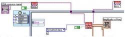
Figure 3. The data acquisition section of the block diagram receives data from the network analyzer. It sets the frequency at which measurements are taken. Additionally, the resonance frequency amplitude versus frequency is outputted to a front panel. This section of the resonance frequency tracking software block diagram is shown above in more detail.
The Colpitts oscillator is an example of a circuit which can be used for the testing of acoustic sensors. In such a circuit, the resonant sensor device is modeled as a resistor, capacitor, and inductor (RLC) (Martin 1991). The inductor models the mechanical inertia, the capacitor models the material stiffness, and the resistor models the vibration dissipation of the sensor. This segment of the circuit sets the frequency of oscillation. The remainder of the circuit consists of a feedback loop which maintains the stability of the oscillations. However, because each sensor is unique in the way it oscillates, this oscillator circuit must be customized for each type of sensor. The elimination of the need for this oscillator circuit enables sensor researchers to conveniently design and test sensor devices without extensive knowledge of electronics.

Figure 4. The for loop in the data organization section of the resonance frequency tracking software block diagram extracts the clustered data into its x and y values of amplitude and frequency. The index of the minimum amplitude is provided to the frequency array for pairing with the frequency at the same index. The data organization section of the resonance frequency tracking software block diagram is shown in detail above.
For testing the software, acetone was dropped onto several types of acoustic wave sensors. Acetone was chosen because of its fast evaporation and its availability.
The change in frequency of the acoustic wave device is related to the change in mass on the surface of the device by the Sauerbrey equation (Sauerbrey 1959):

Equation 1 1492
Where fo is the resonant frequency in Hertz, Δf is the frequency change in Hertz, Δm is the mass change in grams, A is the surface area of the resonator, ρq is the density of quartz, and μq is the shear stiffness of quartz for an AT-cut crystal.
According to Equation 1, when the acetone is dropped onto an acoustic sensor, the resonance frequency should decrease due to the added mass. As the added mass evaporates, the resonance frequency is expected to return to its original value.

Figure 5. The Write to Measurement File VI outputs the inputted minimum frequency versus a time array to a LabVIEW text file. The time array is automatically generated using the system clock. This section of the resonance frequency tracking software block diagram is shown above.
Once validated through testing on various types of acoustic sensors, this software is expected to become a valuable low-cost, versatile tool for acoustic sensor development and testing.
METHODS AND MATERIALS
Design Goals
The goal for the software was to achieve near real-time tracking of resonance frequency versus time to be used in experiments involving acoustic sensors. The definition of real-time was limited to taking at least one reading every ten seconds. To achieve the design goals, the program must take measurements from an HP8753 Network Analyzer, plot resonance frequency versus time in a graph updating in real-time, and record the numerical data to a file.

Figure 6. The front panel provides the interface between the user and the program. It allows the user to easily control the measurement parameters. An example of the front panel while the software is in operation is shown above.
Software Components
Most of the major functions of the program are enclosed in an adjustable timed loop. The top left corner of the loop lists the properties that may be altered. The top entry sets the internal clock to thousands of milliseconds, or seconds. The second entry sets the desired period between the executions of the loop or measurement sampling period. In Figure 2, the period is set so that one measurement is taken every three seconds. The timed loop is started once the instrument selection reaches the Collect Data Virtual Instrument (VI), and the loop is ended when the user stops the program from the front panel. The advantage of using an adjustable timed loop is that each time the program is run the user may choose to update the data points with the maximum frequency, depending upon the number of points used on the network analyzer at the time. The resulting software is made up four components (data acquisition, data organization, writing data to file, and front panel), each fulfilling a design goal.
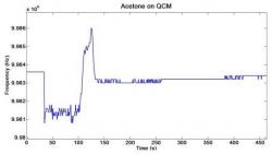
Figure 7. Acetone was hand-pipetted onto the surface of a QCM SAW device. The resonance frequency was tracked as it dropped due to mass loading and returned to its original value as the acetone evaporated. A plot of the resonance frequency versus time after dropping acetone on QCM is shown.
Data Acquisition
Communication with the network analyzer must first be configured using the NI Measurement and Automation Explorer (NI-MAX) software. After the instrument has been configured, the Virtual Instrument Software Architecture (VISA) I/O Selection VI in the top left corner generates a drop-down menu containing a list of connected instruments. The instrument choice is then passed to the Instrument Initialization VI, which opens the interface between the computer and the instrument. The acquired information reaches the Collect Data VI and starts the timed loop. The Collect Data VI acquires the data from the network analyzer in the form of formatted data, and outputs it both on the front panel as an x-y graph displaying amplitude versus frequency, and numerically as an array of clusters of x-y pairs. One component of the clusters contains the x value and the other the y value. This array is then used in the Data Organization section of the program. The Instrument Close VI, shown in the top right of Figure 3, closes the connection with the network analyzer after the timed loop has ended.
Data Organization
The array of x-y clusters are passed to a for loop, which runs for a number of iterations equal to the length of the array, or the number of points in the data set (Knuth 1968). The for loop breaks each cluster apart by passing it to an Unbundle Cluster VI. The outputs of the Unbundle Cluster VI become an array of x-values and an array of y-values upon exiting the for loop. The amplitude y-values are passed to the Array Max and Min VI, shown in the bottom of Figure 4. The frequency x-values are passed to the Index Array VI on the right. The Array Max and Min VI locates the minimum amplitude and its index. It passes the index to the Index Array VI which has the frequency array as the input. The Index Array VI then outputs the frequency with the same index as the minimum frequency. This is the desired resonance frequency of the current data set (the frequency with the minimum amplitude, or the minimum frequency). The resonance frequency is then plotted versus a time value generated by the internal clock in a waveform-graph on the front panel. This is the desired resonance frequency versus time plot. The time between points and the precision may be determined by the frequency at which the timed loop is run.
Writing Data to File
The choice was made to use the Write to Measurement File Express VI for recording numerical data to file; a convenient function with many adjustable options. Figure 5 shows the Write to Measurement File Express VI. The Express VI displays a window, which sets the directory and filename of the saved file. The "Append to File" option in the VI menu was chosen so that each new resonance frequency measurement generated by the iteration of the timed loop creates a new line in the data file. By having the Write to Measurement File VI inside the timed looped and appending to the data file with each iteration, instead of writing the entirety of the data at one time, the program safe-guards against unforeseen computer crashes or other problems resulting in data loss. One header is generated per file with the date and time of measurement and other miscellaneous information. Underneath the header are two columns. One is the time column, containing the time (in seconds) at which each measurement was taken, starting from when the program began running. The other column contains the resonance frequency at each of the times. The measurement file is saved with extension ".lvm", but is a text file that can be exported to a data analysis program such as Microsoft Excel.

Figure 8. Acetone was hand-pipetted onto the surface of a horizontal shear SAW device. It can be seen that the software successfully tracks the resonance frequency. The resonance frequency exhibited the expected outcome of an initial drop followed by a gradual rise back to original value. A plot of the resonance frequency versus time after dropping the acetone is shown above.
Front Panel
On the front panel, shown in Figure 6, the VISA resource name is displayed at the top along with the current minimum frequency, its amplitude, and the time in seconds since the program began running according to the internal clock. The graph on the left is an amplitude versus frequency plot of the acoustic device being measured, transferred from the display on the network analyzer. The graph on the right plots the minimum frequency versus time by taking the x-coordinate of the minimum point on the amplitude versus frequency graph and using it as the y-coordinate versus a computer-generated x-coordinate of time.
Testing
In order to test the software, a drop of acetone was deposited onto three types of acoustic sensors using a hand-pipette. The resulting shifts in resonance frequency were measured with the software to verify its performance and accuracy. The QCM was connected to an HP8753 network analyzer, and a drop of acetone was deposited directly on the QCM. The program ran until the resonance frequency stabilized. The numerical data collected in the measurement file were exported to MATLAB which was used to plot the resonance frequency versus time. A Cascade Summit 9000 probe station was used to take measurements from the other tested devices, and the same procedure was used to collect and process data.
RESULTS
When the acetone was dropped on the QCM, it caused the temperature to drop and added mass to the surface of the sensor. As shown in Figure 7, the resonance frequency of the QCM starts out at approximately 9.9836 MHz and then dropped to approximately 9.9812 MHz after the acetone was dropped onto the sensor. The resonance frequency rebounded to approximately 9.9860 MHz and then finally returned to the original resonance frequency. Figure 8 shows the results of the horizontal shear SAW device tested. Figure 9 shows the results of the longitudinal mode BAW device.
DISCUSSION
The shapes of the frequency shifts of the sensors tested can be explained by mass loading, or the increase of mass on the surface of the sensor due to the drop of acetone (Martin 1991). The increase in mass causes a negative shift in resonance frequency as shown in the Sauerbrey equation (Eq. 1) (Sauerbrey 1959). When the acetone is dropped onto the sensor, the resonance frequency immediately drops sharply from its original value. The resonance frequency then slowly rebounds up to the original value as the acetone evaporates from the device. The rebound of the resonance frequency back to the original frequency may also be attributed to the temperature change upon evaporation of the acetone. The evaporation of acetone decreases the temperature of the sensor. The temperature drop may contribute to the negative frequency shift by affecting the propagation velocity of acoustic waves in the crystal. In the case of the QCM, the resonance frequency overshot its starting value. The cooling effect of the evaporation of acetone may cause the resonance frequency to rebound past its original value until the sensor returns to room temperature. Non-uniform cooling may warp the crystal as the acetone evaporates. Also, the attenuation of acoustic waves through a crystal is proportional to its temperature (Rosenbaum 1945). This contributes to the increase of the resonance frequency above its starting value because the less attenuated acoustic waves propagate faster through the crystal. The temperature then returned to room temperature, and the resonance frequency settled at its starting value. The differences in the rates of frequency rise in the different tests may be attributed to slightly different amounts of acetone being dropped on each device. Because the surface areas of the devices varied considerably, the amount of acetone in contact with the surface was not completely uniform (Campbell 1989).

Figure 9. Acetone was dropped on a longitudinal mode BAW device. The resonance frequency was tracked as the acetone evaporated. The fact that the resonance frequency did not return to its original value may be attributed to the acetone residue left on the surface of the sensor. The plot of resonance frequency versus time after dropping acetone on a longitudinal mode BAW device is shown
CONCLUSIONS
A successful tracking tool was developed for the resonance frequencies of acoustic sensors at a wide range of frequencies without the need for an oscillator circuit. The bandwidth that may be analyzed by the software is only dependent upon the bandwidth of the network analyzer. As seen in the presented results, the software accurately tracks the resonance frequency of different types of acoustic wave devices. It provides a convenient and versatile means of testing acoustic wave devices during development. In the results, the resonance frequency did not return to its starting value in every device after the evaporation of acetone. This may be explained by the presence of a thin film of acetone residue on the surface of the sensor after the acetone has evaporated. This additional mass of the residue suppresses the propagation of acoustic waves in the device, lowering the stabilized resonance frequency. Also, because the way the acoustic waves propagate in each type of device is different, the graph of resonance frequency shifts of each device tested exhibit a different shape. However, each graph shows the same general trend of a resonance frequency drop and rebound after acetone is dropped on the surface of the sensor.
Further improvements may be made to this program by adding the ability to monitor the resonance frequencies of two sensors on two different channels simultaneously, or as close to simultaneously as possible. This would one channel to act as a reference sensor and eliminate common environmental fluctuations by comparing the reactions of the two sensors.
ACKNOWLEDGEMENTS
We would like to thank Dr. William Hunt for being our mentor and providing us the opportunity to work on this project. We also thank Anthony Dickherber and Christopher Corso for their helpful guidance. We would also like to give sincere thanks to Ryan Westafer and John Perng for their willingness to answer questions and help with the project.
REFERENCES
Campbell, C. (1989) Surface Acoustic Wave Devices and Their Signal Processing Applications. Academic Press: San Diego.
Chung, J. W. et al. (2006) Immunosensor with a Controlled Orientation of Antibodies by Using NeutrAvidin-Protein A Complex at Immunoaffinity Layer. Journal of Biotechnology 126: 325-333.
Corso, C. D. et al. (2006) Real-time Detection of Mesothelin in Pancreatic Cancer Cell Line Supernatant using an Acoustic Wave Immunosensor. Cancer Detection and Prevention 30: 180-187.
Corso, C. D. et al. (2007) Lateral Field Excitation of Thickness Shear Mode Waves in a Thin Film ZnO Solidly Mounted Resonator. Journal of Applied Physics 101: 054514.
Knuth, D. E. (1968) The Art of Computer Programming, Vol. 1. Addison-Wesley Professional.
Martin, S. J. (1991) Characterization of a Quartz Crystal Microbalance with
Simultaneous Mass and Liquid Loading. Analytical Chemistry 63: 2272-2281.
Pinkett, S. L. et al. (2002) Determination of ZnO Temperature Coefficients Using Thin Film Bulk Acoustic Wave Resonators. IEEE Transactions on Ultrasonics, Ferroelectrics, and Frequency Control 49: 1491-1496.
Rosenbaum, J. F. (1945) Bulk Acoustic Wave Theory and Devices. Artech House.
Sauerbrey G. (1959) Zeitschrift für Physik 155: 206-222.
Stubbs, D. D. et al. (2005) Vapor Phase Detection of a Narcotic Using Surface Acoustic Wave Immunoassay Sensors. IEEE Sensors Journal 5: 335-339.
Wilson, M. S. et al. (2006) Multiplex Measurement of Seven Tumor Markers Using an Electrochemical Protein Chip. Anal. Chem. 78: 6476-6483.