

Author: Megan Mary Mekarski
Institution: University of Illinois at Chicago
Date: June 2008
ABSTRACT
Understanding the transport and metabolism of 3,4-dihydroxy-L-phenylalanine (L-dopa) in the human brain is necessary to better treat people with Parkinson's disease. This disease is caused by an insufficient amount of dopamine (DA) produced in the brain. Positron emission tomography (PET) imaging has been used to study the activity of the dopamine producing enzyme, aromatic amino acid decarboxylase (dopa decarboxylase), in conjunction with a radio labeled analog of L-dopa, 6-[18F]fluoro-L-dopa or F-dopa. In this paper, using reaction coefficients calculated by Gjedde from PET scans, a set of differential equations representing the mass balance of all the reactions and diffusion from L-dopa to dopamine in the blood and brain was created. The brain was discretized on an unstructured grid based on anatomy so that one can better understand why dopamine concentrates in the midbrain as opposed to peripheral structures. For each volume, three partial differential equations represent the specific balance, one for initial chemical L-dopa, one for the unwanted product methyldopa and one for the end product and its metabolites, dopamine. The results of the simulation demonstrate the grid consistant with behavior of dopamine in human brain which can be observed in the compartment similar to the results of a PET scan of the brain. With this model, the amount of dopamine in a section of the brain at a given time can be found, and the quantities of L-dopa is consumed in the brain to produce dopamine can be better understood.

Fig. 1: Chemical pathways from tyrosine to L-dopa and either to methyldopa or dopamine.
INTRODUCTION
Dopamine is a neurotransmitter and hormone produced from tyrosine in specific neurons located in the midbrain. Fig. 1 depicts the natural pathway of tyrosine in the dopaminergic neurons as it becomes L-dopa and then dopamine or methyldopa. Depending upon the location of the neuron, the dopamine produced there will be released along one of four pathways each with a different outcome. The mesolimbic pathway is associated with feelings of pleasure and desire. This pathway starts in the ventral tegmentum and terminates in the nucleus accumbins in the limbic system. The mesocortical pathway is involved in sending cognitive information to the frontal lobes and connects dopaminergic cells in the ventral tegmentum to the cortex. The nigrostriatal pathway is responsible for inhibiting muscle control. This pathway begins in the substantia nigra and ends in the striatum (which includes the caudate nucleus and putamen). The fourth and final pathway is the tuberoinfundibular which stimulates the release of prolactin by linking the hypothalamus with the pituitary gland (Cooper et al. 1996).

Fig. 2: Schematic of dopaminergic synapse. L-dopa passes through capillary and the blood brain barrier and enters the terminal to be converted into dopamine. The dopamine is then collected in vesicles by VAT. An action potential triggers the natural production of dopamine by phosphorlating tyrosine hydroxylase (TH) and also releases vesicles across the synapse. Dopamine binds to the post synaptic receptors which trigger one of the four pathways depending on their location. When dopamine unbinds it is taken back up into the terminal by DAT or metabolized into DOPAC or HVA which return to circulation for excretion.

The Dopaminergic nerve cells in the nigrostriatal pathway are damaged in the brains of Parkinson's patients causing a loss of dopamine. Without dopamine, these people begin to experience muscle rigidity, tremor, and slowness. Dopamine cannot be administered as a drug because it cannot pass through the blood brain barrier (BBB). The precursor, 3,4-dihydroxy-L-phenylalanine (L-dopa or levodopa), is currently used instead, often in conjunction with carbidopa which prevents the formation of methyldopa (Cooper et al. 1996).
The BBB is responsible for many difficulties in drug delivery not only in Parkinson's disease but among many neurodegenitive diseases that require large molecule drug therapy. The BBB is created by the endothelial cells lining capillary vessels in the brain. The cells are packed together closely, creating tight junctions that only lipid soluble, uncharged and small molecules can pass through without a specific transport system (Kandel et al. 1991). L-dopa is actively transported through the junctions by amino acid transporter (L1) and then converted into dopamine once inside dopaminergic neurons of the brain so it makes a good substitution (Hawkins et al. 2005). Using what is known about L-dopa and Parkinson's treatment, a mathematical model can be developed that will not only improve the delivery of L-dopa but can lead to improvement in delivery of other large molecule drugs that could operate under a similar mathematical model.
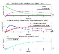
Fig. 4: L-dopa metabolism in a one compartment model of the brain based on five differential equations with some reactions assumed to be negligible.
Once across the BBB, L-dopa is free to diffuse into any part of the brain, but dopaminergic neurons are located primarily in the midbrain. As shown in Fig. 2, L-dopa is taken into the neuron by plasma membrane transporters (DAT), converted into dopamine by dopadecarboxylase (DDC) and collected into vesicles by vesicular amine transporters (VAT). An action potential to the neuron phosphorylates tyrosine hydroxylase (TH) stimulating the natural production of dopamine from tyrosine as well as the release of the dopamine containing vesicles. Dopamine crosses the gap after the nerve ending and binds to post synaptic receptors which will then stimulate one of the four pathways, depending on the location. Some dopamine is reabsorbed by DAT while some is metabolized into 3,4-dihydroxyphenylacetic acid (DOPAC) or homovanillic acid (HVA) (Barrio et al. 1997).
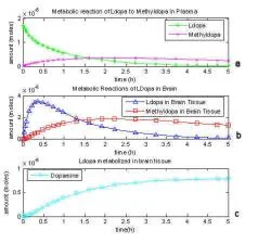
Fig. 5: One compartment model based on Gjedde, 1991, all reactions included.
L-dopa reactions are observed in the brain through positron emission tomography (PET). PET scans measures the total radioactivity of the area scanned in the image. The radiopharmaceutical, 18F, will emit a gamma ray when struck by a positron from the PET. The ray is then absorbed by the scanner to create an image (Kandel et al. 1991). Much like L-dopa, F-dopa can be metabolized into methyl-F-dopa, fluorodopamine, FDOPAC and FHVA. The PET image includes the unwanted byproduct methyl-F-dopa. In order to accurately account for all products in the measurements, the production of methyldopa in the cerebellum (where there are no dopaminergic neurons to produce dopamine) is referenced as background activity to be subtracted out of the total. The methyldopa in the cerebellum can also be used in a ratio to the amount of methyldopa in the striatum (region with caudate nucleus and putamen) to describe the methylated fraction of total radioactivity (Barrio et al. 1997). A detailed description of the mathematics behind interpreting the PET images and calculation reaction coefficients can be found in the appendix.
MATERIALS AND MODEL

Fig. 6: One compartment model of the brain with dopamine metabolites and loss (Deep et al. 1997). Notation from Gjedde, 1991 remains with k7 as the metabolism coefficient of dopamine to DOPAC, k11 as the metabolism coefficient of DOPAC to HVA and k9a and k9b as the loss of DOPAC and HVA, respectively.
Development of Compartmental Model
A compartmental model of the brain was used to study L-dopa's diffusion and metabolism. This method is ideal because different regions of the brain can be separated into compartments based on similar properties and reaction rates. The same chemical reactions can occur in each compartment, but at different rates due to the location and number of corresponding catalysts available. The dopaminergic neurons that naturally produce dopamine from tyrosine are most heavily concentrated in the midbrain. A study of expressed dopamine receptor mRNA has shown that the most receptors are located in midbrain areas such as the caudate nucleus, putamen, and amygdala (Meador-Woodruff 1994). The model should show a greater concentration of dopamine in these regions of the midbrain. Diffusion and reaction coefficients have been calculated from previous PET studies of dopamine in the human brain and will be the backbone of the compartmental model.
The Brain as One Compartment
Gjedde et al. (1991) developed a model of L-dopa's metabolism including both L-dopa and methyldopa in the blood and L-dopa, methyldopa and L-dopa metabolites across the blood brain barrier in the brain tissues. To describe this compartment model shown in Fig. 3, five differential equations are given in Equations 1-5.
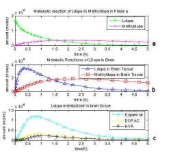
Fig. 7: Graphical representation of a one compartment model including dopamine's further metabolites and loss.

Fig. 8: Regions of interest in PET image of the brain, 5.2cm above the orbito-meatal line (Gjedde 1991).
C1 and C2 are the concentration of L-dopa and methyldopa in the plasma; C3 and C4 are the concentration of L-dopa and methyldopa in the brain tissue and C5 is the concentration of L-dopa metabolites: dopamine, DOPAC and HVA. KD1 is the transport coefficient of L-dopa from the blood plasma across the blood brain barrier to the brain tissue and KD2 is the reverse BBB transport of L-dopa. KM1 is the transport coefficient of methyldopa across the BBB to the brain tissue and KM2 is the reverse transport coefficient of methyldopa across the BBB. KD0 is the reaction coefficient from L-dopa to methyldopa in the plasma and KD5¬ is the reaction coefficient of L-dopa to methyldopa in the brain tissue. KM-1 is the coefficient of clearance of methyldopa from the system. KD3 is the reaction coefficient of L-dopa to dopamine in the brain tissue.
The equations (1-5) contained too many assumptions and deletions, resulting in an inaccurate model of L-dopa metabolite products. For example, the rate of L-dopa to methyldopa in the brain was assumed to be zero, and several other reaction terms became negligible in certain reactions. In Fig. 4, 17 μmoles of L-dopa are initially administered in the plasma. Fig. 4c shows that more L-dopa metabolites have been produced that the original amount of L-dopa administered, reaching about 17 μmoles after three hours and still increasing after, proving it to be an incorrect model.

Fig. 9: Graphical representation of dopamine, DOPAC and HVA combined concentrations in a ten compartmental model of the brain. Concentrations plotted based on the different volumes of the ten compartments.

Fig. 10: Nine compartment model with diffusion showing dopamine, DOPAC and HVA concentration per compartmental volume.
To improve the one compartment model, every reaction from Gjedde's 1991 model (Fig. 3) must be included. When all of the reactions are accounted for the model is represented by Equations 6-10. When these equations are solved, the model seems more accurate, with only half of the original L-dopa ever becoming dopamine or another metabolite (Fig. 5).
Gjedde's work was revisited (Deep et al. 1997; Kumakura et al. 2005) and the model of L-dopa metabolism was improved by including either dopamine, DOPAC and HVA and separate metabolites that eventually leave the system to excretion or still combining them as L-dopa metabolites but incorporating in a loss term. Deep, Gjedde and Cumming's model (1997) model is shown in Fig. 6. The reaction and transport coefficients from the previous model hold the same nomenclature. K7 is the metabolism of dopamine into DOPAC, K11¬ is the metabolism of DOPAC into HVA and K9a and K9b¬ are the diffusion coefficients of DOPAC and HVA respectively out of the system back to circulation to be urinated out. A graphical representation of the second one compartmental model is shown in Fig. 7. Because dopamine (O) can now be depleted from the system, its level does not reach nearly half the original L-dopa dose and remain constant. Instead, it peaks before one hour and does not reach even 10% of the original amount injected. One problem with this model is that the value for K9a¬ could not be measured or calculated, so the value for K9b was used for both terms. For this reason, the kloss value which was introduced by Kumakura (2005) improves the accuracy of the model. Dopamine, DOPAC and HVA can be combined because the level of dopamine is greater than that of its metabolites due to its storage in vesicles before consumption. Dopamine peaked just before 1 hour at 1.2 μmoles where as DOPAC peaked at about the same time with 0.32 μmoles and HVA peaked at 0.21 μmoles.
The Brain in Multiple Compartments, No Diffusion
Different blood brain barrier transport coefficients and L-dopa to dopamine reaction coefficients were measured based on location in the brain and are listed in Table 1 (Gjedde 1991, 2005). Using this data, a multi-compartmental model of the brain was developed with compartments representing the amygdala, midbrain, hippocampus, inferior temporal gyrus, caudate nucleus, putamen, superior frontal gyrus, middle occipital lobe, thalamus and posterior occipital lobe. If this model accurately portrays dopamine diffusion and production within the brain, the most dopamine will be produced in the caudate nucleus and the putamen, followed by other midbrain structures and the least amount of dopamine will be produced out in the occipital lobes and gyruses. A sample PET image from Gjedde's study with regions of interests drawn in is shown in Fig. 8. The two regions on each side with the most 18F pictured are the caudate nucleus and the putamen found directly below.
The first version of a multiple compartmental model included all of the compartments listed above sharing a common blood source with no diffusion between the compartments of the brain. A set of 32 differential equations were developed in the same manor as the previous set, grouping dopamine with its other metabolites, DOPAC and HVA, and including one loss term for simplification.

Fig. 13: Changing the rate coefficient of L-dopa dopamine, KD3.
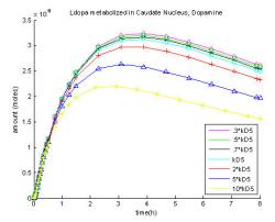
Fig. 14: Changing rate coefficient of L-dopa to methyldopa in the brain, KD5.
The Brain in Multiple Compartments, with Diffusion
Diffusivity coefficients for the tissues of the brain are necessary to account for dopamine diffusion. Since most of the regions of the brain in question are composed of grey matter, a single diffusion coefficient could be used for all of them. The value used in the model was 5.410-4cm3h-1 (Ellegood 2005). Diffusion mass balance equations are based on a concentration gradient between two compartments. In the plane chosen, 5 cm above the orbito-meatal line (Fig. 8) the amygdala cannot be seen. The number of compartments was therefore reduced to nine. Comparative distances and areas were measured and added into the mathematical model. Fig. 10 shows a graphical representation of the diffusion model.
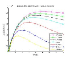
Fig. 15: Changing the rate coefficient of dopamine and its metabolites loss from the system, kloss.
The Brain in Multiple Compartments with Parameter Changes
The reaction rate coefficients can be modified to see how each step affects the production of dopamine and storage of dopamine. By changing various rate constants, adding or removing a certain catalyst can be modeled and the limits can be determined. The reaction rates that were modified are the blood brain barrier transport coefficient of L-dopa, K[SUP]D[/SUP][SUB]1[/SUB] (which in turn changes BBB transport of methyldopa, K[SUP]M[/SUP][SUB]1[/SUB], proportionally), rate coefficient of L-dopa to methyldopa in the blood plasma and in the brain, KD0 and KD5, respectively, rate coefficient of L-dopa to dopamine and other metabolites, KD3, and the metabolism and loss of dopamine, kloss¬. Each reaction rate will be multiplied by 0.2, 0.5, 0.7, 2, 5, and 10.
People taking L-dopa for their Parkinsonism will often require more than one dose per day. In this paper we will show how dopamine is lost in the system after a second dose is given at a particular time. Fig. 16 shows the same 17 μmole amount being added after four hours, and how slowly it is metabolized, even after ten hours. Currently, Sinemet, a popular drug, is administered to patients in pills with carbidopa to L-dopa ratios of 1:4 and 1:10. The two different pills are prescribed in different amounts over the course of a few weeks until the best ratio has been determined ("Sinemet (Carbidopa-Levodopa)" 2002).
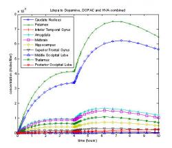
Fig. 16: Ten compartment model with diffusion and a second L-dopa dose after four hours

Fig. 17a: Computational Unstructured Grid. Fig. 17b: Brain structures assigned to grid compartments. Caudate Nucleus (red), Putamen (orange), Thalamus (yellow), Hippocampus (green), Midbrain (blue), Superior Frontal Gyrus (brown), Inferior temporal gyrus (purple), Middle occipital lobe (mint green), posterior occipital lobe (pink).
The Brain in Two Dimensions
A computational unstructured grid (Fig. 17a) was drawn to mimic a horizontal slice of the brain 5cm above the orbito-meatal line. In nature, the brain is a distributed system. The grid contained 179 compartments. For each compartment, three equations were assigned: one for diffusion and loss of L-dopa, one for diffusion, production and loss of methyldopa, and one for diffusion, production and loss of dopamine and further metabolites. Properties of structures in the brain were assigned to the compartments as shown in Fig. 17b. The equations were originally written using an equation generator that matched each compartment with an x and y position as well as writing diffusion equations based on the distance between the center points of adjacent compartments. The equations were then edited to each occur three times, with the reaction and blood brain barrier transport terms for L-dopa, methyldopa or dopamine added on to one of each triplet. The program that graphed the brain plotted the concentration of one or all or the chemicals involved for compartment on the x,y scale. Fig. 18a shows the concentration of L-dopa in the brain after two hours. Fig. 18b shows the concentration of methyldopa in the brain after two hours. Fig. 18c shows the concentration of dopamine in the brain after two hours and Fig. 18d shows the concentration of all three species summed together in the same way that a PET scan would show the total radioactivity and display F-dopa, methyl-F-dopa and fluorodopamine in the same image.

Fig. 18a: L-dopa in the brain two hours after initial injection of 17 µmoles to the blood. Fig. 18b:Methyldopa in brain after two hours. Fig. 18c: Dopamine in brain after two hours. Fig. 18d: Sum of L-dopa, methyldopa and dopamine in brain after two hours.
METHODOLOGY
The models were solved using MATLAB and the ode15s ordinary differential equation solver. Differential equations were developed in Equation 11, where kz is the reaction coefficient of substance m becoming substance n in a particular compartment or the diffusion coefficient of substance n entering the compartment from compartment m and kb is the reaction coefficient of substance n becoming another substance or substance n leaving the compartment. CLDPlasma and CMDPlasma represented L-dopa and methyldopa in the blood source, respectively. The L-dopa in the plasma is lost to methyldopa production (KD0¬), blood brain barrier transport (K[SUP]D[/SUP][SUB]1[/SUB]) and gained by transport back across the BBB from the brain tissue (KD2) as described in equation (12). The methyldopa in the plasma is lost from the system (KM-1) and lost across BBB transport (K[SUP]M[/SUP][SUB]1[/SUB]) and added from L-dopa (KD0) and from the brain across the BBB (KM2) as shown in equations 12 and 13.
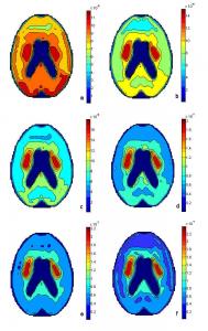
Fig. 19a: Sum of L-dopa, methyldopa and dopamine and metabolites after 30 minutes. Fig. 19b: Sum of L-dopa, methyldopa and dopamine and metabolites after 60 minutes. Fig. 19c: Sum of L-dopa, methyldopa and dopamine and metabolites after 90 minutes. Fig. 19d: Sum of L-dopa, methyldopa and dopamine and metabolites after 120 minutes. Fig. 19e: Sum of L-dopa, methyldopa and dopamine and metabolites after 150 minutes. Fig. 19f: Sum of L-dopa, methyldopa and dopamine and metabolites after 180 minutes.
Each compartment in the brain then receives three more equations: one representing L-dopa in the particular compartment, methyldopa in the compartment, and dopamine, DOPAC and HVA combined in that compartment. L-dopa enters a brain compartment from the plasma across the blood brain barrier (K[SUP]D[/SUP][SUB]1[/SUB]) and is lost back across the BBB (KD2), to the production of dopamine (KD3), and to the production of methyldopa (KD5) as written in equation (14). Methyldopa enters a brain compartment by transport across the BBB (K[SUP]M[/SUP][SUB]1[/SUB]) or production in the plasma (KD5) and is lost back across the BBB (KM2) as shown in equation (15). Dopamine, DOPAC and HVA are produced in a brain compartment from L-dopa (KD3) and is removed from the system with a collective loss term (k¬loss) as described in equations 14-16.
Dopa metabolites (dopamine, DOPAC and HVA) can be combined because the output of DOPAC and HVA is much less than dopamine, and the clearance coefficient of DOPAC, K9a could not be determined experimentally so using a new parameter, kloss, more precisely portrays the reactions in the compartment from dopamine on.

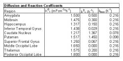
Table 1: Diffusion and Reaction Coefficients based on location in the brain.
To add diffusion to the model, equation (11) was modified, where D is the diffusivity constant, C(n) is the concentration in the compartment in question, C(p) is the concentration either diffusing in or out of the compartment and delta(x) is the distance between the centers of two compartments. If there is a higher concentration in compartment m, then the chemical in m will diffuse into n and vise versa. The equations are completed by including every production and loss term, plus diffusion between all adjacent compartments. In the compartmental model, each triplet of equations (14-16) sharing a compartment had the same set of diffusion terms added on; one for each neighboring compartment.
RESULTS

Equations 1-8
One Compartment
The first draft of the one compartment model shows the levels of L-dopa and methyldopa in the blood plasma and L-dopa, methyldopa and dopa metabolites in the brain tissue. Fig. 4a reports 17 μmoles of L-dopa (*) initially administered in the plasma of the model. The level of L-dopa in the plasma decreases as some of it becomes methyldopa (X) and some diffuses across the BBB. Methyldopa levels in the blood plasma reached 7.57 μmoles before clearance overtook production at two hours. Fig. 4b depicts a sharp increase in L-dopa (Δ) as it first passes the BBB into the brain tissue. L-dopa peaked at 6.16 μmoles before 45 minutes have passed. The supply is continuously depleted as some of it becomes methyldopa (□) and some goes on to produce dopamine and other metabolites (O). The methyldopa levels in Fig. 4b also begin to decrease after three hours when it was 3.92 μmoles since it is diffusing out of the system to be later excreted. Fig. 4c shows that more L-dopa metabolites have been produced that the original amount of L-dopa administered, reaching about 17 μmoles after three hours and still increasing after to 21.5 μmoles at six hours, proving it to be an incorrect model.
When all of the reactions up until the production of dopamine are considered, the dopa metabolite level is now less than the original introduction of L-dopa as shown in Fig 5. After four hours dopa metabolites reached 7.82 μmoles and began to level off.

Equations 9-17

Equations 18-29
Including further metabolism of dopamine plus loss shows how dopamine leaves the brain tissue as it is consumed to produce DOPAC (+) and HVA (◊) which will be excreted through urination as shown in Fig 7. This addition to the one compartment model completes the mass balance of equations. Dopamine only reached 1.18 μmoles at 45 minutes and DOPAC peaked at 0.31 μmoles and HVA maxed at 0.21 μmoles.
Mulitple Compartments
Breaking the model into ten compartments proves that dopamine concentrates in the midbrain regions due to the location of specific enzymes and receptors that produce dopamine. The greatest amounts of dopamine were produced in the putamen, caudate nucleus, and thalamus, which are all located in the midbrain. When these compartments are compared by volume, the highest concentrations exist in the putamen (X), followed by the caudate nuclueus (O). The other midbrain regions: the amygdala (*), midbrain (□), thalamus (star), and hippocampus (diamond) had a concentration about one quarter of the caudate or putamen. The outer regions: inferior temporal gyrus (+), superior frontal gyrus (downward arrow), middle occipital lobe (delta) and posterior occipital lobe (six-pointed star) all had very low concentrations, with the occipital lobes never producing dopamine and always at zero. The most dopamine per compartmental volume was found in the putamen at 0.42 μM after three hours, followed by the caudate nucleus reaching 0.39 μM after three hours (Fig. 9). Next, were the midbrain, the amygdala, the thalamus and the hippocampus peaking at 0.090 μM, 0.090 μM, 0.065 μM, and 0.041 μM respectively after two hours (Fig. 9). Very little or no dopamine was produced in the inferior temporal gyrus, superior frontal gyrus, the posterior occipital lobe and the middle occipital lobe, which were all found to be below 0.017 μM.
Adding diffusion to the model (Fig. 10) reverses the top two, with the highest concentration in the caudate nucleus with a maximum of 0.20 μM followed by the putamen which reached 0.17 μM. These maximums were reached after three hours. The next highest concentration was the thalamus, reaching 0.067 μM after two hours. The other six regions, hippocampus, midbrain, superior frontal gyrus, inferior temporal gyrus, middle occipital lobe and posterior occipital lobe never reached 0.01 μM of dopamine and metabolites. Adding diffusion to the model reduces the total amount of dopamine made per compartment because L-dopa can diffuse out of the striatum before dopamine can be produced. The comparative volumes also are based on fractional areas in a plane rather than total volumes in the three dimensional space.
Changing Parameters
When the rate constant of active transport across the blood brain barrier, K[SUP]D[/SUP][SUB]1[/SUB], was reduced the amount of dopamine produced decreased. When K[SUP]D[/SUP][SUB]1[/SUB] was augmented, dopamine production increased, but was limited As shown in Fig. 11, the curve showing dopamine production when K[SUP]D[/SUP][SUB]1[/SUB] was multiplied by a factor of 2 is the same as the curve when K[SUP]D[/SUP][SUB]1[/SUB] was multiplied by 5 and 10 by a difference of less than 2%. Only the graph for the caudate nucleus is shown in Fig. 16 but the other nine compartments were tested and showed the same results.
Increasing KD0, the coefficient of methyldopa production in the blood plasma greatly reduced dopamine production. In the caudate nucleus (Fig. 12), the maximum dopamine production was reduced by 54.4% to 0.0014μM when the rate constant was increased tenfold. Reducing the coefficient of methyldopa production in the blood to thirty percent of its original only increased dopamine production by ten percent.
Increasing the rate of L-dopa metabolized into dopamine was limited in the caudate nucleus and the putamen, where production of dopamine was already high. Fig. 13 shows that when the coefficient KD3 was multiplied by 5 the curve is the same as when it was multiplied by 10. A t-test performed on the two sets relayed a value of 1.36E-4%, proving that the data sets are the same.
The rate coefficient of methylation in the brain tissue used was 0.05 h-1, which is very low when compared to the other reactions in the brain and plasma. Since the value is so small, it does not heavily influence the production of dopamine. As shown in the Fig. 14 where the curves for KD5, 0.7*KD5, 0.5*KD5, 0.3*KD5 are all within 4% of each other, reducing the rate of L-dopa methyldopa in the brain doesn't significantly increase the amount of dopamine.
Fig. 15 shows the dopamine levels as the rate of their loss from the system, kloss is increased or decreased. When the rate of loss is increased ten times dopamine level peaks at an hour and fifteen minutes at 0.0014 μM, which is 45% of the original maximum. When the loss of dopamine and metabolites is slowed to thirty percent of the rate of loss, dopamine reaches its maximum at a later time, at five hours and thirty minutes, and comes to 0.0037 μM which is 17% greater than the original.
The second dose model shows how dopamine levels are maintained in Parkinson's patients during the day. As shown in Fig. 16, a second dose of L-dopa of the same magnitude as the original is administered after four hours, which is when the dopamine levels of the first dose peak. More dopamine is made and three hours after the second dose consumption overtakes production beginning a slow drop in dopamine levels.
Two Dimensional Compartmental Model
The two dimensional model shows how the three species: L-dopa, methyldopa, and dopamine concentrate in the brain. Fig. 18a, shows L-dopa in the brain two hours after the 17 µmole dose of L-dopa was administered in the blood. L-dopa has equal probability of diffusing across the blood brain barrier to every compartment in the unstructured grid since capillaries are everywhere in the brain. Low concentrations, between 0.038 μM and 0.051 μM of L-dopa exist in the caudate nucleus and the putamen because L-dopa is being lost to dopamine production. Higher concentrations, ranging from 0.070 μM to 0.089 μM of L-dopa are found in the occipital lobes because the posterior occipital lobe and middle occipital lobe have the two highest values of K[SUP]D[/SUP][SUB]1[/SUB], the active transport constant of L-dopa across the blood brain barrier, as shown in Table 1. Notice that the maximum concentration of L-dopa is 0.089 µM. In Fig. 18b, the production, loss and diffusion of methyldopa is shown two hours after the initial dose of L-dopa. Methyldopa also has an equal chance to be transported across the blood brain barrier to any section of the brain. The graph shows an equal distribution across the plane of the brain with some build up along the edges due to the boundary conditions preventing diffusion outside of the brain except back to the blood system. The concentration of methyldopa ranges from 0.0085 μM to 0.0097 µM. The third graph, Fig. 18c, shows the production of dopamine from L-dopa as well as its diffusion and loss from the system. The highest concentrations of dopamine are found in the caudate nucleus and putamen where dopamine was found at 0.15 μM with very low concentrations in other midbrain regions with a local maximum at 0.036 μM and no dopamine produced or diffused to the outside regions. The fourth graph, Fig. 18d, is the summation of L-dopa, methyldopa and dopamine and mimics a PET scan which displays total radioactivity and would be showing F-dopa, methyl-F-dopa and Fluorodopamine in the same image. Just like the PET Scan in Fig. 8, Fig. 18d shows a high concentration in the caudate nucleus and putamen, up to 0.20 μM, half the straitum concentrations were found in the midbrain, 0.10 μM, and 0.08 μM found along the outer regions.
The sum of all species with respect to time is shown in the series of graphs in Fig. 19. The images were taken in intervals of 30 minutes for three hours. In Fig. 19a, 17 μmoles of L-dopa was added to the blood source 30 minutes prior and accounts for most of the picture with a maximum of 0.09 μM since it has been transported across the BBB to the volumes of the grid. Methyldopa is occurring evenly across the distributed system but at a smaller scale, with a maximum at 0.003 μM or 3 nM. In three hours, methyldopa concentrations never exceed the nanomolar scale so its contribution to the total graphs is negligible. Dopamine production has already begun after 30 minutes and the highest concentration in the total picture is found in the striatum. The dopamine concentration in the caudate nucleus and the putamen is 0.05 μM. Dopamine is not the most abundant specie in the brain after 30 minutes but its combination with L-dopa in the striatum accounts for the high concentration in that region. Fig. 19b shows the sum of all species after an hour. L-dopa is still copious with a maximum of 0.09 μM after sixty minutes. The maximum level of dopamine is also 9 μM after an hour. With only half of the maximum L-dopa level occurring in the caudate and putamen, the highest concentration found in Fig. 19b is in the caudate and putamen reaching 0.14 μM. Fig. 19c is the sum of all species after 90 minutes. The supply of L-dopa is beginning to deplete and its maximum is now 0.08 μM. Dopamine and its metabolites, on the other hand, are rapidly produced and stored so in the striatum the concentration reaches 0.12 μM. This leads to a maximum in Fig. 19c of 0.18 μM. Fig. 19d is the sum of L-dopa, methyldopa and dopa metabolites after two hours have passed. L-dopa is still being consumed after 120 minutes so its maximum is down to 0.07 μM. Dopamine has reached 0.14 μM after two hours. The maximum in Fig.19d occurs once again in the striatum and is 0.20 μM. Fig. 19e depicts the sum of all species after 150 minutes. L-dopa has been depleted to a maximum 0.06 μM and dopamine in the striatum has increased to 0.16 μM after two hours and thirty minutes. The maximum concentration in Fig. 19e occurs in the caudate nucleus and the putamen at 0.23 μM. Fig. 19f represents the sum of L-dopa, methyldopa and dopamine and its metabolites after three hours have passed since the initial introduction of L-dopa to the blood system. L-dopa consumption is still occurring and its maximum is down to 0.05 μM. Dopamine production is also taking place after three hours and the concentration in the caudate nucleus and the putamen has reached 18 μM. The maximum concentration in Fig. 19f, the sum of all species after three hours, occurs in the caudate nucleus and the putamen at 0.24 μM.
DISCUSSION AND CONCLUSIONS
The ten compartment model of the brain based on thirty-two simultaneously solved differential equations is an accurate portrayal of L-dopa's behavior after being introduced to the circulatory system. L-dopa and methyldopa have the ability to diffuse from capillaries into any section of the brain, but dopamine is only produced where the necessary enzymes and receptors are located. The receptors are in place to complete one of the four pathways with the striatum being a major ending point in the nigrostriatal pathway. The highest concentrations of dopamine and its metabolites can be found in the caudate nucleus and putamen as a result. Nearby structures, the amygdala, midbrain, thalamus and hippocampus all produce dopamine and therefore had significant concentrations, although not as high as those found in the striatum. Very little dopamine was produced in the gryruses and none in the occipital lobes. It was only until diffusion was added into the model that any dopa metabolites were found in the middle occipital lobe and the posterior occipital lobe. Because the diffusion coefficient is so small, the amount of dopamine reaching those areas is still negligible, showing that dopamine concentrates in the midbrain due to the production centers in the dopaminergic neurons, not diffusion characteristics.
Changing the parameters has created a better understanding of how the various reactions involved affect the production of dopamine. Increasing the blood-brain barrier transport constant (Fig. 11) will increase dopamine production, but L-dopa to methyldopa is the rate limiting step so increasing the active transport coefficient by a factor of two is equivalent to increasing the coefficient by five or ten. When the rate constant of methylation in the blood plasma is increased dopamine production will be greatly decreased (Fig. 12). Currently, methyldopa is produced in the blood plasma at about a third of the rate of L-dopa being transported across the BBB. Increasing methyldopa output reduces the amount of L-dopa available to be transported across the BBB and then metabolized into dopamine. Increasing the rate of dopamine production in the brain led to increased dopamine production that was only limited in the caudate nucleus and the putamen where concentrations are high already. The curves for 5 * KD3 and 10 * KD3 in Fig. 13 passed a t-test proving the curves are statistically not different. The rate of methylation in the brain tissue is very low compared to the other reactions involved so when it was reduced the production of dopamine was not affected, as shown in Fig. 14. The curves for KD5, 0.7 * KD5, 0.5 * KD5, and 0.3 * KD5 are all within 4% of each other. If dopamine is not stored in vesicles it will be metabolized quickly. In Fig. 15 the value for kloss, the rate constant for dopamine's metabolism and loss from the system, was changed. An increase in the rate of removal resulted in a great decrease in dopamine with the maximum dipping to 45% of the maximum of dopamine and metabolites before the loss term was modified. Decreasing the removal rate increased the amount of dopamine and metabolites stored up to 17% more than the original.
In the two dimensional compartmental model, L-dopa (Fig. 18a) is shown with its lowest concentrations found in the caudate nucleus and the putamen. L-dopa has been consumed in the striatum for dopamine production. The highest levels of L-dopa were found in the posterior occipital lobe and middle occipital lobe. The active transport constant across the blood brain barrier is highest in those two regions. Methyldopa was produced and distributed evenly at low levels throughout the brain. Methyldopa can diffuse across the BBB to any compartment and can be produced in any compartment, which explains its distribution. Dopamine can only be produced in the midbrain, primarily the striatum. Dopamine is produced and then stored in vesicles, so the levels do not drop off quickly as opposed to the clearance of methyldopa from the system. Dopamine that diffuses out of the striatum is consumed quicker than in due to storage vesicles only being in dopaminergic neurons. The dopamine levels are greater than any other species in the system due to its storage.
When the sum of all species (Fig. 18d) is compared to a PET scan (Fig. 8), it is apparent that the highest concentrations occur in the caudate nucleus and the putamen in both images. The maximum dopamine concentration is twice that of the maximum L-dopa concentration and an order of magnitude higher than the highest methyldopa concentration. Subtracting out the activity in the cerebellum from the whole PET image and assuming it to be L-dopa and methyldopa is an appropriate method of viewing dopamine only because both occur at a narrower range than dopamine and its metabolites. A single value can therefore be assumed to represent both species and still leave an accurate image of dopamine distribution in the brain.
The sum of all species with respect to time (Fig. 19a-f) is a dynamic representation of the sort of data a PET scan would produce. A series of images would be collected and analyzed to better understand how 18F-dopa is transported and metabolized in the human brain just as the simulation can produce a series of images showing how L-dopa is transported and metabolized on the unstructured grid. The sequence (Fig. 19a-f) illustrates the sum of the species starting out with a distribution throughout the brain and then concentrating in the striatum while elsewhere the total of the species is depleted. This action is similar to the occurrences in live human brain as shown by PET imaging and demonstrates the accuracy of the mathematical model.
The two dimensional model is a good representation of L-dopa's transport and metabolism in the human brain. As expected, the highest concentrations of dopamine are found in the caudate nucleus and the putamen, where dopamine is produced. Some dopamine is produced in other midbrain regions, but that amount is very small and nearly negligible when compared to the caudate and the putamen. L-dopa and methyldopa each have equal chance to distribute to any compartment in the brain from the blood, so their distributions are near even. L-dopa and methyldopa can also pass across the blood brain barrier from the brain back to the blood, so it may exit the system that way. Dopamine can only leave the system if it has been metabolized into DOPAC or HVA. The kloss value in the caudate and putamen (0.078 h-1 and 0.098 h-1, respectively) is much smaller than the blood brain barrier transport constant elsewhere (3.23 h-1 for L-dopa, 7.43 h-1 for methyldopa) because dopamine is stored in vesicles before use and further metabolism. This storage is show in my model as dopamine is found in concentrations an order of magnitude greater than L-dopa and methyldopa which can more readily leave the system.
The compartmental model of dopamine in the brain can be used in drug therapy planning for Parkinson's patients. With this model, doctors will know how quickly a particular dosage will diffuse and be metabolized. They can plan when another dosage is needed by seeing at what time the dopamine level has dipped too low. The model is also capable of predicting a second dose at a particular time and will show how dopamine levels will change over time and the dosage amounts and time can be optimized for a particular patient.
ACKNOWLEDGEMENTS
I would like to thank the REU supplement, NSF-DMI-0328134 grant, for funding my research this summer. I would also like to thank Professor Andreas Linninger for his advice and knowledge and Dr. Libin Zhang for all his guidance.
REFERENCES
Barrio J, Huang S, Phelps M. Biological Imaging and the Molecular Basis of Dopaminergic Diseases. Biochemical Pharmacology 1997; 54: 341-348.
Cooper, Jack R., Floyd E. Bloom, and Robert H. Roth. The Biochemical Basis of Neuropharmacology. 7th ed. New York, NY: Oxford University Press, 1996.
Deep P, Gjedde A, Cumming P. On the accuracy of an [18F]FDOPA compartmental model: evidence of vesicular storage of [18F]flourodopamine in vivo. Journal of Neuroscience Methods 1997; 76: 157-165.
Gjedde A, Reith J, Dyve S, Leger G, Guttman M, Diksic M, Evans A, Kuwabara H. Dopa decarboxylase activity of the living human brain. Proc Natl Acad Sci USA 1991; 88: 2721-5.
Ellegood J, Hanstock C, Beaulieu C. Trace Apparent Diffusion Coefficients of Metabolites in Human Brain using Diffusion Weighted Magnetic Resonance Spectroscopy. Magnetic Resonance in Medicine 2005; 53: 1025-1032.
Hawkins, Richard A.; Mokashi, Ashwini; Simpson, Ian A. An active transport system in the blood - brain barrier may reduce levodopa availability. Experimental Neurology 2005; 195(1): 267-271.
Hoffman, Beth J., Hansson, Stefan R., Mezey, Eva, Palkovits, Miklós. Localization and Dynamic Regulation of Biogenic Amine Transporters in the Mammalian Central Nervous System. Frontiers in Neuroendocrinology 1998; 19: 187-231.
Kandel, Eric R., Schwartz, James H., Jessell, Thomas M. Principles of Neural Science. 3rd ed. New York, NY: Elsevier, 1991.
Kumakura Y, Vernaleken I, Grϋnder G, Bartenstein P, Gjedde A, Cumming P. PET studies of net blood-brain clearance of FDOPA to human brain: age dependant decline of [18F]flourodopamine storage capacity. Joural of Cerebral Blood Flow & Metabolism 2005; 25: 807-819.
Meador-Woodruff J, Damask S, Watson S. Differential expression of autoreceptors in the ascending dopamine systems of the human brain. Proc. Natl. Acad. Sci USA 1994; 91: 8297-8301.
Seeman P, Van Tol H. Dopamine receptor pharmacology. Trends in Pharmacological Sciences 1994; 15: 264-270.
Warner, Joseph J. Atlas of Neuroanatomy: With Systems Organization and Case Correlations. Boston, MA: Butterworh Heinmann, 2001.
APPENDIX
Calculating Reaction coefficients from PET scans
To be more accurate in differentiating the fluorescing species in the PET image, the concentrations can be determined mathematically. Fig. 3 shows the model of L-dopa reactions Gjedde proposed in 1991. The first box, C1, represents the concentration of L-dopa in the blood plasma. L-dopa in the blood can become methyldopa in the blood in C2 or diffuse across the blood brain barrier into C3. L-dopa in the brain can also become methyldopa, C4, diffuse back across the blood brain barrier, C1, or be converted into dopamine, DOPAC and HVA which are summed in C5. The total 18F introduced to the body equals the sum of all the radiolabeled species in the blood and brain, as shown in Equation 18.
C1 and C2, the concentrations of L-dopa and methyldopa in the blood, will not show up in the PET scan. Instead, they are measured by High Performance Liquid Chromatography (HPLC). The rate constant of methlyation, KD0, and the clearance of methyldopa constant, KM-1 can be determined by linearizing the relationship between L-dopa and methyldopa in the blood, as shown in Equations 19 and 20.
The experimental results of HPLC can be plotted linearly, as shown in Fig. 20 with KD0 as the slope and -KM-1 as the intercept.
To solve equation (18) for rate coefficients in the brain, the sum of radioactivity in the blood, C1 + C2 can be replaced by C* multiplied by the volume of distribution in the blood, V0. The concentration of dopamine and further metabolites, C5, will be dropped initially to solve for the diffusion of L-dopa across the blood brain barrier, K[SUP]D[/SUP][SUB]1[/SUB], and Ve, the partition volume which equals K1¬/k2. The solutions of C3 and C4, equations (3) and (4), respectively, are Equations 21 and 22.
When q is a previously determined constant equaling the ratio between L-dopa's diffusion across the blood brain barrier and methlydopa's diffusion across the blood brain barrier, equation (18) becomes Equation 23.
The partition volume, Ve¬, can now be determined.
To make the equation more accurate and to solve for K[SUP]D[/SUP][SUB]1[/SUB] and KD3, the reaction coefficient of L-dopa to dopamine in the brain, the rate of change of L-dopa in the brain is modified in Equations 24 and 25.
The solution to equation (5) is simply Equation 26.
But equation (25) must be substituted into (26) so that C5 is in terms of knowns C1 and C2, as shown in Equations 27 and 28.
When substituting (22), (25) and (28) into (18), the result is Equation 29.
The coefficients K[SUP]D[/SUP][SUB]1[/SUB], KD3 and the volume of distribution in the blood, V0 can be solved for.